
Background
The horse racing community has been using quantitative data to develop betting algorithms for decades. Indicators including horse bodyweight, age, and previous lap times are all utilized along with the domain-specific Speed Index to predict future race outcomes. Our team was asked to answer a new question in horse racing: Can subjective data taken by an SME improve the predictive ability of horse racing models?
Our partner in this task was RaceQuant, a horse racing syndicate that makes proprietary wagers on races in Hong Kong’s two venues: Happy Valley and Sha-Tin. Prior to each race, participating horses are walked around an open area next to the track known as the ‘paddock.’ Racing insiders stand by and orate their observations of each horse to a respective betting syndicate. RaceQuant had contracted an SME to take note of specific features, and One Hot Encoded the observations. These observations can include subjective takes like ‘confident’ or ‘nervous,’ and seemingly span the entire English vocabulary. For the study, features were broken down to between 5 and 7 distinct values. As an example, some horses will have bandaged legs. This feature would then be broken down into categories of [front-leg single, front-leg double, rear-leg single, rear-leg double, all] and subsequently One Hot Encoded for data privacy. The observations spanned one season of racing and 800 individual races.
In addition to the features provided by the SME, all observations also included which one of the 23 primary trainers was the trainer for the horse. Features indicating the rank of each horse by bodyweight in the race were given, as well as columns indicating how the horse’s bodyweight had changed since its prior race. As with the data provided from the Paddock, the trainer and bodyweight data was One Hot Encoded.
In order to judge the relevance of the provided data, RaceQuant established two benchmarks: The Tips Indexes provided by the Hong Kong Jockey Club and the Odds data for each horse in each race. The Tips Indexes provided by the Hong Kong Jockey Club are published on its website at www.hkjc.com before 4:30 pm on the day preceding a race day and before 9:30 am on each race day morning. For the analysis, the team utilized the race day measure of the Tips Index. “A Tips Index is not a "tip" itself but a reference figure based on selections by the racing media and generated by applying a statistical formula. Each starter's Tips Index represents the degree of favor it has among tipsters. For easy comprehension, a Tips Index is expressed in the form of an odds-like figure. The smaller the figure, the higher is the degree of favor a starter enjoys among tipsters.” Historically, the Tips Indexes ~24% of the winning horses.
The Odds data was taken five minutes prior to the start of the race. Odds are subject to change and are fully correlated with the amount of money placed on the horse. Additionally, the true odds payout is not set until the start of the race. Consequently, the value of a ticket purchased can move up and down accordingly. Lastly, the racetrack collects ~22% of total wagers as commission. Therefore, the summed probabilities of winning for the horses racing is 1.22 or 122% as derived from the listed odds. Historically, the Odds favorite wins ~33% of the time.
RaceQuant had two primary questions regarding the data: First, can the Paddock data alone or in conjunction with the Tips Index and Odds be used to predict a higher percentage of winning horses relative to the established benchmarks on an “unseen” number of races. Second, would a model using this data provide a higher ROI than the benchmarks after making one unit bets on the model’s favored horse over a given period of time.
With two benchmarks to compare results, the team focused on probabilistic classification models to decide whether or not a horse is a winner. A motivating factor in this decision was that the RaceQuant desired full transparency in the models so future efforts could focus on features with statistically significant results. Given this, along with the limited data, the agreed upon choice was to utilize Logistic Regression models in the research. Bolton and Chapman had already proven the usefulness of a multinomial logit model for handicapping horse races in their 1986 white paper. However, given the highly subjective features within the data set the team also developed a Random Forest Classifier.
An obstacle was the nature of the data, more specifically, that the models lacked the ability to identify the ‘race-by-race’ nature of the data. This meant each horse would effectively be racing against all of the horses in the dataset, including itself if there were > 1 observations. To solve this problem, we pulled the win probabilities each model assigned a given horse, and then ranked the horses in a given race based on the model-assigned probability of winning.
To summarize, two models were trained, a Logistic and Random Forest classifier, for both the Paddock data alone and the combined Paddock and Tips/Odds dataset. For the test set, the probabilities of winning for each horse were determined from the models, and the expected winner of each race was selected as the horse with the highest win probability. The total number of correct predictions was calculated, and the picks from our models on the test set were compared with our two benchmarks: betting on the horse with the most favorable odds and betting on the horse with the most favorable Tips Index.
Results
When the Logistic Regression and Random Forest were trained and tested on only the Paddock dataset, these models underperformed their benchmarks. Moreover, the return (loss) from utilizing strictly the Paddock data performed no better than random selection.
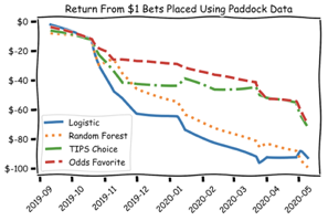
While all four strategies seem to track closely for the first two months, eventually both models diverge and never recover. Between November and December of 2019 the random forest outperforms on the test set. These results may simply be noise, as this deviation is well within the critical value to have appeared at random. Nevertheless, there does appear to be structure within the results that tracks in line with the Tips and Odds dataset; specifically in January, late March, and early May.
One of the first decisions on how to proceed with the analysis was whether to use the Tips Index, the Odds favorite or both as comparative indexes. To answer this, the first step was to determine whether or not there was a statistical difference in the performance of the Odds favorite as compared to the Tips favorite. Using Fisher’s exact test, the team determined that performance results are dependent on the proxy used with a p-value of 0.00032 and a higher return for the Tips Index.
While strictly utilizing the Tips Index in the model may have led to enhanced initial performance, the decision was made to include both; the team hoped that any divergence between the Tips Index and the Odds favorite may be of value to the model.
Promising results were observed when the Paddock data was supplemented with the Odds and Tips Index of each horse.
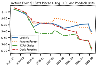
In the same timeframe, both the Logistic Regression and Random Forest classifiers made selections that resulted in smaller losses than the benchmarks. Additionally, the win rate of each model had a significant increase. Single unit bets made only on the TIPS favorite accurately predicted the winner in 22.6% of the test races, while betting only on the odds favorite accurately predicted the winner in 26.4% of the test races. Logistic Regression, however, predicted 28.3% of the winners while Random Forest predicted 28.9%. Additionally, the models were able to track the better performing index, rising as Tips returns diverged from Odds in November, and increasing again in February as Tips returns turned upwards.
Based on Fisher’s exact test it can be concluded that performance is, in fact, dependent on the selection strategy of the models against both the Tips index and Odds favorite. While additional data will be needed for a higher level of confidence, it appears that the Paddock data is, in fact, a confounding variable which leads to enhanced prediction accuracy and reduces overall loss under a one unit betting strategy.
To determine the efficacy of the model’s strongest predictions, four thresholds [60%, 70%, 80%, 90%] were implemented, and the model was run against each. Each test required the model’s choice to have a predicted win probability at or above the threshold in order to place a wager. If no horse in a race exceeded the threshold then no bets were placed.
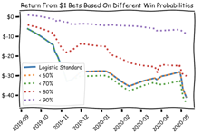
While changing the threshold did not result in a profitable model, the model with > 90% only exhibited loss due to the racetracks commission on each bet placed. Another interesting takeaway was that the >70% model actually underperformed the base model. This highlights the value of correctly selecting horses in well-matched races as well as long-shots to drive ROI.
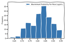
A major concern from this analysis was the distribution of the probability to win for the horses selected by the model to win a respective race. That is, how frequently a horse with probability to win of x had the highest percentage chance, as predicted by the model, to win its race. The most frequent observations occurred between ~80% and ~87.5%. Working backwards, this yields a break-even odds (when using 85%) of 3/17 (1.18 in decimal and -566.67 American/moneyline).
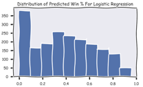
It is clear that the model’s win percentage predictions are substantially higher than in reality. The primary cause of this problem was the binomial nature of the modeling. When the win probabilities from the Logistic model are graphed for all horses, a large number of horses are given virtually no chance to win the race. As the expected win probability increases past 5%, a peak is seen at ~35% followed by a steady drop-off. However, even with the steady drop-off sufficient horses exhibit the features of a “winning” horse to receive a high probability. As the project moves forward and a multinomial is exchanged, these probabilities will decline.
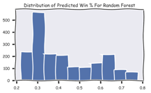
Interestingly, the Random Forest classifier had more difficulty in identifying strictly losing horses. The Random Forest classifier also had fewer ambiguous values (those between 40% and 60%). While neither of the models produced promising distributions based on implied odds, the logistic model captured more distinctly “losing” characteristics. Moving forward, the Kelly Criterion, also known as the scientific gambling method, will take these probabilities as inputs and allocate funds accordingly. Until these probabilities are brought in line, no asset allocation can be completed.
Takeaways
The initial challenge faced surrounded the data itself. While the TIPS Index dataset spanned five years, the Paddock data only included observations for one season of racing. This limited our observations to only 800 races ~ 8000 observations in total and 1414 distinct horses.
Given the focus on strictly predicting horses that finished first, the team elected to develop a baseline model using only the data provided and compare the results to strategies of selecting winners using the TIPS Index and predictions made by the “wisdom of crowds” inherent in the Odds favorite. This choice was made to a large extent so that the results could be clear to the client, and the team would be able to present options of how to remedy issues that were encountered in the data. As this project would eventually be moved to an internal team, transparency around decisions was vital.
While the model did outperform both indexes, the sensitivity of the models required significant improvement before they could be implemented. The need for more observations was clear.
Several techniques could have been used to increase observations of the minority class in this situation. However, within the horse racing community there are domain-based practices of resampling with origins based in the Ranking Choice Theorem developed by Luce and Suppes (1965). More recently, Chapman and Stalin have described how “the extra information inherent in such rank ordered choice sets may be exploited and provided an“explosion process” that applies to a class of models of which the stochastic utility model is a member. By applying the Chapman and Stalin explosion process, it is possible to decompose rank ordered choice sets into ‘d’ statistically independently choice sets where ‘d’ is the depth of explosion. Bolton and Chapman’s “Searching For Positive Returns At The Track” provides the example of three such sets: “[horse 4 finished ahead of horse 1, 2, and 3], [horse 2 finished ahead of horse 1 and horse 3], and [horse 1 finished ahead of horse 3], where no ordering is implied among the “non-chosen” horses in each “choice” set.”
These exploded choice sets are statistically independent, so they can be easily added to the dataset and are equivalent to completely independent horse races. This leads to an increase in the number of independent choice sets available for analysis and, ultimately, would provide more precise parameter estimates. “Extensive small-sample Monte Carlo results reported in Chapman and Stalin document the improved precision that can accrue by making use of the explosion process.” This becomes tremendously valuable due to both the time and cost of obtaining a sufficiently robust dataset to use for modeling.
Due to the limited amount of quantitative data, feature engineering appeared to be a prescient path to take in order to bolster prediction accuracy. Average lengths distance behind the winner appeared to be a good starting point. For horses that won, this number would be the negative lengths between the horse and second place. However, the frequency distributions of races ran by a horse are heavily right-skewed, as many have run only one race. Additionally, this metric would be biased against horses that have never run before. In a random forest model, this issue could be slightly mitigated by using a dedicated large number to represent such horses but for the logistic model, a solution could not be so easily implemented. However, there were several remedies available:
- Utilize available metrics such as Speed Index (when available) to predict the horse’s finish time at the race distance and ensemble the two models
- Identify the horse in the current dataset with > n finishes most similar to the horse in question using KNN and assume the same value for the variable
- Average the horse’s past n performances during training over the same distance
Given that the data for use did not include quantitative metrics other than the number of lengths that a horse placed behind the winner the only applicable solution was to use KNN. However, the implementation of such a technique over all the variables in the dataset might not actually be necessary in this situation. It has already been discussed that bodyweight, trainer, and jockey are important variables from the Paddock dataset. The team’s hypothesis is that adding readily available information such as Speed Index, which is known to have a strong correlation to finish time, might be enough to estimate the average range of time that a horse would take to finish a race. Testing this theory using AIC or BIC over the aforementioned variables and additional variables from the Paddock dataset would be a very informative next step.
After analyzing the average lengths behind the winner data the team saw a fairly frequent trend of high variance in horses that finished below fourth place. Even winning horses would have runs that had a drastically negative impact on their average distance to the winner. The thesis behind this variability was that once a jockey knew his/her horse would not place the jockey would ease off of the horse and reserve as much of the horse’s energy for another race or for training. When the filter was applied so that only the top four horses were accounted for on each race, the standard deviation fell by over 62%. Because of this, the team was back to not only the first question of how to manage horses that have not run but also how to manage horses that have not placed in the top four. Several approaches were presented on how to manage this issue. The first was to One Hot Encode various distance gaps and add an additional label to signify a placing below fourth. To accomplish this task would require a SME who could validate the methodology and additional statistical analysis.
Before delving into such an undertaking, the team decided to track whether or not wins-to-races ran as well as places-to-races ran was a strong indicator of future performance. The team did this by separating the training and testing dataset by race date and then calculating total races won to total races for all horses in the training set. These numbers were then applied to each horse in the testing set with unseen horses receiving a value of zero.
The result of this approach was a higher predicted win probability for horses with a high index but a drop-off in total accuracy due to the bias against unseen horses. Additionally, because of the rules of racing in Hong Kong, dominant horses may have additional weight added in subsequent races. The model was unable to account for these changes.
Overall, the team concluded that additional quantitative information is necessary to effectively utilize feature engineering for the model. While the Paddock data alone performed no better than a random choice approach, when coupled with the TIPS and Odds data the Paddock observations appear to act as a confounding variable that substantially increase overall model returns. Nevertheless, due to the lack of observations and subsequent variance observed in the model, the team would need to gather more data to establish a definitive stance.
Sources:
'Searching For Positive Returns At The Track: A Multinomial Logit Model For Handicapping Horse Races" Bolton & Chapman 1986
www.hkjc.com The Hong Kong Jockey Club
Topics from this blog: Capstone