Team Machine Learning Project

A quick introduction

Kaggle is a sort of data science candyland in which one can pick and choose from almost any data set imaginable. Kaggle is also a website that allows for Data scientists to compete against each other to see which models are most effective and predicting a certain feature. Though the competition was closed, our team’s goal was to predict the housing prices of Ames, Iowa by submitting our models to the public leaderboard.  This was an exciting opportunity because such information can be quite useful. Real Estate agents, bankers, home buyers, and home sellers could all make use of knowing the most powerful predictive features identified by the most successful models.

Data Described

The data was composed of 80 variables. Seventy-nine of those features were predictor features. These features ranged from categorical variables such as the neighborhood that the house was sold in to primarily quantitative variables such as the square footage of the first floor.  The target feature was the quantitative variables, sale price, in U.S. dollars.  The data was pre-split into a training set and a test with each set being given in the form of a csv file. This totaled to 1460 rows on the training set and 1459 rows for the testing set (- minus the sale prices).

Data Visualized

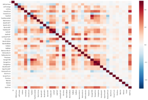
It’s always great to start with a correlation plot. You can see here that the features most strongly related sale price are, not surprisingly, the overall quality and GrLivArea (which is). The features most related to each other are the year it was built / year the garage was built and the first floors square feet and the total basement square feet.We really did not find this as a surprise at all.

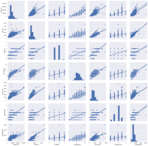
The graph below represents the features that seem to have strong linear relationships of the data in greater detail. The scatterplot visualization allows you to see the linearity of the data and the degree of variance each feature has. Linear features follow the line of best fit such is in the case of case of overall quality predicting sale price. Although linear, this corrplot appears to vary more than total square footage and predicting basement square footage since the data points don’t appear to cluster as much around the mean. Perhaps total square footage and total basement square footage can be collapsed into one variable. Overall this is a very nice visualization that gives a more detailed explanation of the relationship between the features.

 Scatter Plot

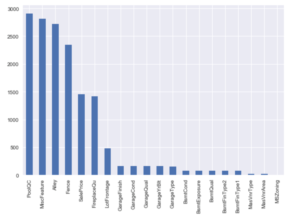
The two graphs below represent missing data. The first graph represents the data that has the most missing values. The second graph is merely an extension of the first graph. Don’t be deceived by the size of the bars in the graphs. The highest bar representing pool QC represents over 2500 missing values. The highest bar in the second graph, MSC zoning, represents only 4 missing values.  Some of these missing values are actually not missing at all. They represent they lack some value such as the case of fences. It's not that there are no records of missing fences. It is the fact that there are not any fences surrounding certain homes. This fact will play a major role in how the data should be cleaned in the project. Another interesting thing to note regarding missing data is the case of missing garages.

Features with a lot of missing values.

Features with only a few missing values.

Data Cleaned and Fun

The first task was to identify which features where quantitative. Categorical features were imputed in python by changing NA values into the most common value. Ex: data.loc[all_data.Alley.isnull(), 'Alley'] = 'NoAlley'.

'BsmtUnfSF'] = house_all.BsmtUnfSF.median()

'BsmtFinSF1'] = house_all. BsmtFinSF1.median()

Only one is null and it has type Detchd?

Only one is null, guess it is the most common option WD?

Many columns have missing values, and not all can be treated the same way. Some are missing because they are just not applicable to the house in question (e.g. columns giving info about fireplaces/pools/garages for houses which do not have those things). The rest of the numerical values were imputed with the mean or median.  Imputing allows for feature transformations. Feature transformation is critical for meeting the assumptions of several models including ridge and lasso regressions. One assumption of these models is that features are normally (bell curve) distributed with data points being clustered around the mean.  The Y variable must first be transformed.

It was found that the original sale price was skewed to the right but that the log transformation (log + 1 of sales price) did an excellent job of centering the data around the mean. Lastly some of the categorical variables needed to be dummified to incorporate them into the regression model. The process of dummification involved converted categories into 1 or 0 based on whether a condition was true or not. If the house had a garage, then it would be assigned a 1 value. If it did not have that value, then it would be assigned a zero. This allowed of the data to be incorporated into regression models since all the data was now numeric.

SKEWNESS_CUTOFF = 0.75

'SaleCondition'] = 'Normal'

The data of course must be split back from the train to the test set.

Once the data had been thoroughly cleaned we could attempt feature engineering to see if there was a way to improve a model’s prediction in any way. “YrSold” and “MoSold” although numbers were categorical variables and were changed accordingly. As mentioned in the data visualization section, it appeared that a lot of the square footage variables were related to each other. This would make common sense because you would expect the floors of the house to have a similar amount of square feet. It would be unlikely to have a significantly larger second floor relative to the first floor.  Living Area Square Footage (Total_Liv_AreaSF) was the combined features of 1stFlrSF, 2ndFlrSF, LowQualFinSF, and GrLivArea.  Our hypothesis is that reducing these similar features into one would reduce the complexity of the model(s) and thereby improve overall predictions.

Models tested

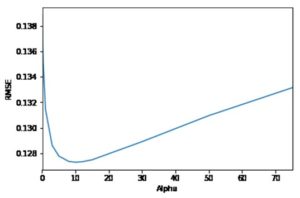
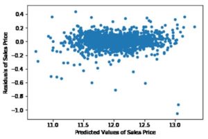
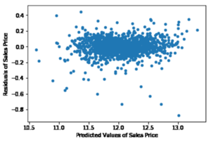
We officially chose one model 4 models to test although one of team members dabbled with XGboost. Each of the models was broken into 5 folds with the 5th fold reserved for testing and the rest for training. Our initial hypothesis was that the tree-based models (gradient boosting and random forest) would be most successful at predicting sales prices but we chose to use the ridge and lasso regression since because they would be easiest to interpret and because we are still learning.  The ridge and lasso regression are generally better than the simple linear model because they introduce a regularization parameter. This allows for the model to avoid overfitting due to an increased complexity (number of features in this case). Overfitting will result in higher variance. Our team must reduce that variance by introducing such parameters since many features can certainly an issue. The main reason behind our group using Ridge Regression was because of the model’s ability to alleviate multiple collinearity or the independence of each variable. Too much multicollinearity can result in an overwhelming amount of variance and destructive overfitting.  Our best prediction from the Ridge regression was having the root mean squared error of .12623 and the alpha (regularization parameter) being of .10. We found that for the most part that the residuals were centered around the mean. This meets the assumption of having relatively independent errors.

Lasso model is useful because of its tendency to prefer solutions with fewer parameters. This is because the Lasso eliminate features that don’t have any value regarding the prediction. Certain variables such as RoofMatl_Metal and Street_Pave were totally eliminated from this particular model.

Tree-based models are advantageous because they do not assume linearity. You don’t need to meet as many assumptions as for the linear models when attempting to predict a variable. Decision trees tend to rapidly overfit, so we chose to use the more complex models in Random Forests and in Gradient Boosting. Random Forest is effective at dealing with a large number of features since it automatically selects which features are the most significant features at predicting the target value. Random forest works by randomly sampling from each feature or bagging.  In our case, our RMSE was .14198 with min samples per leave being 1 and the minimal split per tree being at 4 The maximum number of features is 67 and the random state remained at zero. You can see the number of features below.

Gradient boosting “learns” by improving on each decision tree by minimizing the number of residuals. We chose to use Gradient boosting because it frequently outperforms random forest models. Post cross-validation, our optimal parameters were having a learning rate of “0.05", a max depth of 5, minimum samples split of 4, and the number of estimators being at 1000.  Our tuned model contained an RMSE of 0 .12916.

Conclusion

Our original goal was to find the best model to predict housing prices in Ames, Iowa. Our initial hypothesis was incorrect. The linear models turned out to be the most effective at predicting house prices. In particular, the Lasso model proved to be the most effective at prediction with a RMSE of 0.12290. This is likely the most effective model because it was able to drop the unnecessary variables and because linear models tend to work fine with fewer rows/columns of data. Future paths of research would be to limit the number of features to reduce complexity in tree based models

Also potentially forge Principal Components to reduce complexity by reducing the number of dimension.Also finding more ways to effectively feature engineer through gaining a better grasp on Real Estate in this area