Take Me Out to the Ballgame: Predicting MLB Attendance (with Web Scraping & Shiny)

Contributed by Michael Todisco. He is currently in the NYC Data Science Academy 12 week full time Data Science Bootcamp program taking place between January 11th to April 1st, 2016. This post is based on his thirds class project - Web scraping and Shiny (due on the 6th week of the program).

Michael Todisco

Overview

Is there anything better than going to a baseball game?  Provided it's during the day, sunny, above seventy degrees,  on a Saturday, and there's a free hat giveaway for the first 30k fans.  The point being that there are many factors that go into a fans decision to show up to the ballpark.  My goal for this project, was to explore these variables with historical attendance data and make a prediction on the game-to-game attendance totals for the New York Yankees upcoming season.

Getting the Data

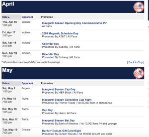
The majority of the data was very easy to obtain using Baseball-Reference's Play Index tool.  The site has robust data that dates back to the 1800's.  However, one aspect of the project that I was emphatic on including was promotional data.  This refers to a teams pre-game promotions such as a hat or bobble-head giveaway.  This data is not tracked on Baseball-Reference.  The only place I could find it was on the New York Yankees official website and it only dated back to 2009.  Furthermore, the data could not be downloaded, but instead I would have to scrape the calendars.

Web Scraping

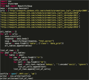
The promotional data I needed was in the form of calendars.  I decided to use Python and Beautiful Soup to do the scraping and after inspecting the elements of the website, it didn't seem like  it would be too much trouble to gather the information.

However, I ran into an immediate wall when I realized the calendars were interactive and written with Javascript.  After a lot of searching for solutions,  I found Dryscrape, which allowed me to access the text.  Once I had that in place, it only took a few simple 'for' loops and appending to lists.  Finally, I wrote the scraped data to a .csv file.

Preparing the Data

Once I had my scraped promotional data and the main dataset from Baseball-Reference, I decided to load them into R.

nyy_scraped = read.csv('nyy.csv')
yankees = read.csv('Yankees.csv')

There were a few column manipulations and additions that I made.  Below is one example, which adds in the opponent's league column.

###Adding Column For Opponent's League###
AL = c('Baltimore Orioles', 'Boston Red Sox', 'Chicago White Sox', 
       'Cleveland Indians', 'Detroit Tigers', 'Houston Astros', 
       'Kansas City Royals', 'Los Angeles Angels', 'Minnesota Twins', 
       'New York Yankees', 'Oakland Athletics', 'Seattle Mariners', 
       'Tampa Bay Rays', 'Texas Rangers', 'Toronto Blue Jays')

league_func = function(x){
  if(x %in% AL) return('American League')
  else
    return('National League')
}

yankees$Opp_league = sapply(yankees$Opp, league_func)

The main step I needed to do with the data was to merge the scraped dataset with the data I downloaded from baseball reference.  I did this using 'Date' as the key.

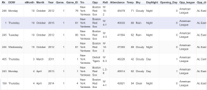
yankees = merge(yankees, nyy_scraped, by = 'Date', all.x = TRUE)

Here's a shot of some of the data in the app.

Building the Shiny App

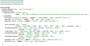
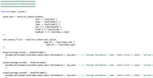
With the data collected and prepared, my next step was to build the interactive tool using Shiny.  With Shiny, it is necessary to create a front-end UI.R file, along with a back-end Server.R file.  The two working together provide the interactive functionality.  Below are a small snapshot of each, but the full code can be found here.

UI.R                                                                                                                    Server.R

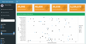
Here is a shot of the main tab/graph of the Shiny App.

The functionality and features that I built into the Shiny App were the following:

• Attendance Visualizations by:
  • Season
  • Opponent
  • Day of the Week
  • Month
  • Particular game
• Visualizations can be filtered by:
  • Game time (day v. night)
  • Temperature
  • Weather
  • Promotion (yes v. no)

The graphs and value boxes - average, maximum and minimum attendance - update as each filter is changed.

Attendance Analysis

The best thing about Shiny and its interactive functionality is that there are endless amount of filter combinations to filter within the tool.  In addition, a user can freely gather insights on overarching trends or get information as granular as a single game.  The average attendance for games against the Orioles, on Tuesdays nights, with a promotion running and temperatures in the mid 50's, is only a few clicks away.

Here are a few of the high-level insights that I was able to take away.  Some are fairly straight forward and common sense, but others are quite interesting.

• Day games have, on average, higher attendance numbers than night games.  For example, in 2013 average attendance for day games was 42k and for night games it was 39k.  This was surprising to me, but I figured out that it was largely due to the next point.
• Weekend games bring in more fans than weekday games.  This makes sense since people typically have off work and to the first point, most of the Saturday and Sunday games take place during the day.
• Temperature and weather have little effect on the attendance numbers, especially when the Yankees have a good record and are in the playoff-hunt towards the later part of the season, when weather tends to be less friendly to fans.
• The Yankees ran promotions for roughly 30-40% of their home games.  Last year promotions did show an uptick of about 2k extra attendees compared to games when promotions were not run.
• Total attendance over the entire season has been steadily declining since 2009, where total attendance was 3.8 million compared to 2015 at 3.2 million.

Prediction Model

The MLB 2016 schedule is of course already out and the Yankees have also released their promotional calendar for the upcoming season.  Using this information and the past data that I was able to build the Shiny App, I was able to fit a model to predict attendance numbers for the 2016 season.

I used the below simple multiple linear regression model to regress attendance on to six variables.

train.model = lm(Attendance ~ Opening_Day + Month + DOW + DayNight + Opp + Promo, data = yankees.train)

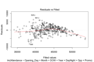
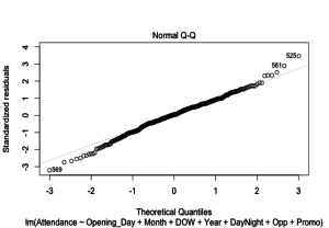
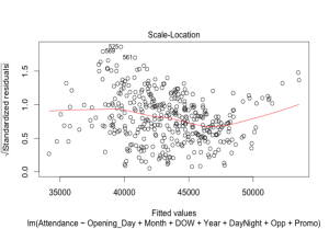
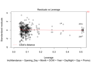
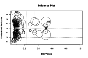
Because this is a linear regression model, it was necessary to graphically check that the model is not violating linear assumptions such as Linearity, Normality, Constant Variance, and Independent Errors. I also check outliers and influence points.

The graphs aren't perfect and there is definitely some areas to be concerned with, but for the most part I can accept this model as adhering to the assumptions of linear regression.

Cross-Validation with training and test sets for the model was performed with the following code:

#Train and test set
set.seed(0)
training_test = c(rep(1, length = trunc((2/3) * nrow(yankees))),
                  rep(2, length = (nrow(yankees) - trunc((2/3) * nrow(yankees)))))
yankees$training_test = sample(training_test) #random permutation
yankees$training_test = factor(yankees$training_test,
                               levels = c(1,2), labels = c("TRAIN", "TEST"))
yankees.train = subset(yankees, training_test == 'TRAIN')
yankees.test = subset(yankees, training_test == 'TEST' & Month != 'March')

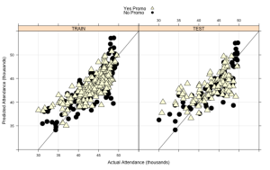
Here is a visual of the accuracy of the model on the training and test sets:

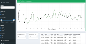
I graphed the models y-variable (Attendance) on a season long plot in the Shiny App on its separate tab.  A user can select a specific game or a range of games to view their attendance.

There is a lot about the model and predicted attendance that looks promising.  The highest predicted games for the yankees occur on Saturday day games against the rival Boston Red Sox and Baltimore Orioles.  Games with low estimated attendance occur on Tuesday nights and do not involve a promotion.   However, there will undoubtedly be error in the regression and it will need to be tuned moving forward.

Conclusion

I was very pleased with how this project turned out.  I combined a myriad of aspects of data science that I have learned in this bootcamp; R, python, web scraping, machine learning and Shiny.  Shiny is a really useful and well designed tool that I will continue to utilize in my projects and work moving forward.

Next steps for this project include scraping the rest of the MLB promotional  calendars so that I can include every team and not just the Yankees.  I also wan to train more accurate/complex models to predict the attendance numbers for the 2016 season.  While multiple linear regression is easy to understand and interpret, I believe a more sophisticated supervised learning technique will yield better results.