R And The Search For Another Earth
Intro
For this project, my goal was to analyze the NASA Exoplanet Archive dataset in order to predict the likelihood that a Kepler Object of Interest (KOI, potential planet) is indeed a planet.
Background
Before getting into the detail of my analysis, some background information will be helpful. The data I used for this project comes from the NASA Exoplanet Archive. NASA does a good job at describing the archive. The following is from the archive's "About" page, http://exoplanetarchive.ipac.caltech.edu/docs/intro.html :
The NASA Exoplanet Archive is an online astronomical exoplanet and stellar catalog and data service that collates and cross-correlates astronomical data and information on exoplanets and their host stars and provides tools to work with these data. The Exoplanet Archive is dedicated to collecting and serving important public data sets involved in the search for and characterization of extrasolar planets and their host stars. The data include stellar parameters (such as positions, magnitudes, and temperatures), exoplanet parameters (such as masses and orbital parameters) and discovery/characterization data (such as published radial velocity curves, photometric light curves, images, and spectra).
Basically, the website host a large dataset that contains all kinds of information about KOIs. This information ranges from easy-to-interpret variables, such as planetary mass and radius, to obscure and hard-to-interpret variables such as fit parameters from various astrophysical models. Here is a link to the page explaining what all the different variables mean: http://exoplanetarchive.ipac.caltech.edu/docs/API_kepcandidate_columns.html. These variables are obtained through multiple experiments and models and formed into an aggregate set. The most important variable in the dataset is the KOI Disposition, which has values of "Candidate", "Confirmed", and "False Positive". These values indicate the Kepler Missions determination of whether a KOI is indeed a planet or a false positive. The "Candidate" value indicates that a KOI has not been confirmed as a planet or a false positive. So, this dataset seems perfect for training a logisitic regression model using the data points with a KOI Disposition of "Confirmed" and "False Positive" as the training set. Then, once the model is built, the KOI Disposition of data points with a KOI Disposition of "Candidate" can be predicted to be either "Confirmed" or "False Positive". This analysis could be used to select "Candidate" KOIs for confirmation that have a high probability of being "Confirmed". This is beneficial because in order to confirm these KOIs as planets, satelite or ground-based telescopes must use up their finite and expensive resources to double check these KOIs. By double checking the KOIs with the highest probability of being "Confirmed" NASA can cut down on the effective cost per planet confirmation/discovery.
Analysis
To begin my analysis, I first had to download the KOI Cumulative List data set, which can be found here: http://exoplanetarchive.ipac.caltech.edu/cgi-bin/TblView/nph-tblView?app=ExoTbls&config=cumulative. I cheated a little and opened the .csv file in excel and cleaned it up some before importing to R. Once imported into R, I looked at the summary.
## randomForest 4.6-10
## Type rfNews() to see new features/changes/bug fixes.
## Loading required package: grid
## Loading required package: mvtnorm
## Loading required package: modeltools
## Loading required package: stats4
## Loading required package: strucchange
## Loading required package: zoo
##
## Attaching package: 'zoo'
##
## The following objects are masked from 'package:base':
##
##     as.Date, as.Date.numeric
##
## Loading required package: sandwich
## Loading required package: sgeostat
## Type 'citation("pROC")' for a citation.
##
## Attaching package: 'pROC'
##
## The following objects are masked from 'package:stats':
##
##     cov, smooth, var
#import data
all = read.csv("keplerData3.csv")
kepler = read.csv("keplerData3.csv")
#summary of data
summary(kepler)## koi_disposition koi_period koi_depth
## CANDIDATE :3185 Min. : 0.24 Min. : 5.9
## CONFIRMED : 993 1st Qu.: 3.56 1st Qu.: 195.8
## FALSE POSITIVE:3170 Median : 11.26 Median : 471.9
## Mean : 78.12 Mean : 15301.5
## 3rd Qu.: 43.15 3rd Qu.: 1301.7
## Max. :129995.78 Max. :961488.0
## NA's :284
## koi_duration koi_impact koi_incl koi_sma
## Min. : 0.250 Min. : 0.0000 Min. : 6.88 Min. : 0.00580
## 1st Qu.: 2.399 1st Qu.: 0.1505 1st Qu.:85.94 1st Qu.: 0.04400
## Median : 3.645 Median : 0.4073 Median :88.81 Median : 0.09205
## Mean : 5.130 Mean : 1.1874 Mean :83.43 Mean : 0.22077
## 3rd Qu.: 5.975 3rd Qu.: 0.8220 3rd Qu.:89.95 3rd Qu.: 0.21862
## Max. :93.160 Max. :100.9710 Max. :89.95 Max. :44.98920
## NA's :284 NA's :284 NA's :284
## koi_dor koi_ror koi_prad
## Min. : 0.91 Min. : 0.00228 Min. : 0.14
## 1st Qu.: 7.26 1st Qu.: 0.01330 1st Qu.: 1.42
## Median : 19.07 Median : 0.02164 Median : 2.29
## Mean : 85.86 Mean : 0.77384 Mean : 132.07
## 3rd Qu.: 51.56 3rd Qu.: 0.05537 3rd Qu.: 7.91
## Max. :79614.00 Max. :99.98200 Max. :109061.00
## NA's :284 NA's :284 NA's :284
## koi_teq koi_steff koi_slogg koi_srad
## Min. : 25.0 Min. : 2661 Min. :0.146 Min. : 0.116
## 1st Qu.: 522.8 1st Qu.: 5324 1st Qu.:4.332 1st Qu.: 0.816
## Median : 820.5 Median : 5787 Median :4.466 Median : 0.963
## Mean : 986.0 Mean : 5714 Mean :4.370 Mean : 1.445
## 3rd Qu.: 1241.2 3rd Qu.: 6131 3rd Qu.:4.554 3rd Qu.: 1.164
## Max. :14225.0 Max. :11086 Max. :5.283 Max. :149.058
## NA's :284 NA's :284 NA's :284 NA's :284
## koi_smass ra dec koi_kepmag
## Min. :0.0940 Min. :279.9 Min. :36.58 Min. : 6.966
## 1st Qu.:0.8330 1st Qu.:288.5 1st Qu.:40.77 1st Qu.:13.530
## Median :0.9690 Median :292.2 Median :43.72 Median :14.601
## Mean :0.9902 Mean :292.0 Mean :43.83 Mean :14.328
## 3rd Qu.:1.0770 3rd Qu.:295.9 3rd Qu.:46.73 3rd Qu.:15.344
## Max. :3.6440 Max. :301.7 Max. :52.34 Max. :20.003
## NA's :284
## koi_gmag koi_rmag koi_imag koi_zmag
## Min. : 7.225 Min. : 7.101 Min. : 7.641 Min. : 7.657
## 1st Qu.:14.014 1st Qu.:13.479 1st Qu.:13.371 1st Qu.:13.346
## Median :15.143 Median :14.553 Median :14.373 Median :14.302
## Mean :14.903 Mean :14.284 Mean :14.132 Mean :14.047
## 3rd Qu.:15.971 3rd Qu.:15.298 3rd Qu.:15.084 3rd Qu.:14.960
## Max. :21.150 Max. :19.960 Max. :19.900 Max. :17.403
## NA's :32 NA's :8 NA's :107 NA's :460
## koi_jmag koi_hmag koi_kmag koi_count
## Min. : 5.393 Min. : 4.854 Min. : 4.718 Min. :1.000
## 1st Qu.:12.330 1st Qu.:11.988 1st Qu.:11.919 1st Qu.:1.000
## Median :13.293 Median :12.892 Median :12.806 Median :1.000
## Mean :13.050 Mean :12.673 Mean :12.596 Mean :1.461
## 3rd Qu.:13.994 3rd Qu.:13.579 3rd Qu.:13.509 3rd Qu.:2.000
## Max. :17.372 Max. :17.615 Max. :17.038 Max. :7.000
## NA's :21 NA's :21 NA's :21
## koi_insol koi_srho koi_model_snr koi_fpflag_nt
## Min. : 0 Min. : 0.0001 Min. : 1.00 Min. :0.0000
## 1st Qu.: 18 1st Qu.: 0.3526 1st Qu.: 14.30 1st Qu.:0.0000
## Median : 107 Median : 1.3860 Median : 27.45 Median :0.0000
## Mean : 5396 Mean : 12.8930 Mean : 215.16 Mean :0.1179
## 3rd Qu.: 562 3rd Qu.: 3.8115 3rd Qu.: 78.30 3rd Qu.:0.0000
## Max. :9678287 Max. :989.5966 Max. :12808.40 Max. :1.0000
## NA's :284 NA's :284 NA's :284
## koi_fpflag_ss koi_fpflag_co koi_fpflag_ec koi_ldm_coeff1
## Min. :0.0000 Min. :0.00000 Min. :0.0000 Min. :0.1161
## 1st Qu.:0.0000 1st Qu.:0.00000 1st Qu.:0.0000 1st Qu.:0.3250
## Median :0.0000 Median :0.00000 Median :0.0000 Median :0.3717
## Mean :0.1116 Mean :0.08628 Mean :0.1076 Mean :0.3964
## 3rd Qu.:0.0000 3rd Qu.:0.00000 3rd Qu.:0.0000 3rd Qu.:0.4488
## Max. :1.0000 Max. :1.00000 Max. :1.0000 Max. :0.9122
## NA's :284
## koi_ldm_coeff2
## Min. :-0.1135
## 1st Qu.: 0.2375
## Median : 0.2814
## Mean : 0.2617
## 3rd Qu.: 0.3005
## Max. : 0.4467
## NA's :284After a quick glance at the summary, I removed some outliers and found some near zero variance variables.
#clean data up
kepler$koi_disposition = as.character(kepler$koi_disposition)
kepler = kepler[kepler$koi_prad < 30000,]
kepler = kepler[kepler$koi_srad < 50,]
kepler = na.omit(kepler)

#remove near zero variance variables
idx = 1
tempList = numeric(0)
for (i in 2:length(kepler[1,])){

  if (var(kepler[,i]) < .5){

    tempList[idx] = i
    idx = idx + 1

  }
}
Then, I remove the near zero variance variables and create various data partitions for the modeling and graphing. I split the data into two main sets. "trainingSet" contains all the "Confirmed" and "False Positive" data points, and the "newSet" set contains the unconfirmed "Candidate" data points. Furthermore, I randomly split the training set into train, validation, and test sets. Finally, I made a centered and scaled copy of all the different data splits and converted the response variable to 0 or 1.
#create a centered and scaled dataset
keplerCS = kepler[,-tempList]
kepler = kepler[,-tempList]

keplerCS = data.frame(scale(keplerCS[,-1], center = TRUE, scale = TRUE))
keplerCS = cbind(koi_disposition = kepler$koi_disposition, keplerCS)
keplerCS$koi_disposition = as.character(keplerCS$koi_disposition)

#separate out training validation test and new sets
newSet = kepler[kepler$koi_disposition == "CANDIDATE",]
trainingSet = kepler[kepler$koi_disposition != "CANDIDATE",]
newSetCS = keplerCS[keplerCS$koi_disposition == "CANDIDATE",]
trainingSetCS = keplerCS[keplerCS$koi_disposition != "CANDIDATE",]

indices = sample(1:length(trainingSet[,1]), size=length(trainingSet[,1]),
                 replace = FALSE, prob = NULL)

fullSet = trainingSet
fullSetCS = trainingSetCS

testSet = fullSet[indices[1:700],]
finalSet =  fullSet[indices[701:1400],]
trainingSet = fullSet[-indices[1:1400],]

testSetCS = fullSetCS[indices[1:700],]
finalSetCS =  fullSetCS[indices[701:1400],]
trainingSetCS = fullSetCS[-indices[1:1400],]

test_koi_disp = ifelse(testSet$koi_disposition == "CONFIRMED", 1, 0)
testSet$koi_disposition = test_koi_disp

train_koi_disp = ifelse(trainingSet$koi_disposition == "CONFIRMED", 1, 0)
trainingSet$koi_disposition = train_koi_disp

full_koi_disp = ifelse(fullSet$koi_disposition == "CONFIRMED", 1, 0)
fullSet$koi_disposition = full_koi_disp

test_koi_dispCS = ifelse(testSetCS$koi_disposition == "CONFIRMED", 1, 0)
testSetCS$koi_disposition = test_koi_dispCS

train_koi_dispCS = ifelse(trainingSetCS$koi_disposition == "CONFIRMED", 1,0)
trainingSetCS$koi_disposition = train_koi_dispCS

full_koi_dispCS = ifelse(fullSetCS$koi_disposition == "CONFIRMED", 1, 0)
fullSetCS$koi_disposition = full_koi_dispCS
Next, I need to find an optimal subset of predictor variables to feed to the model.
#find best subset of predictors
subs <- regsubsets(koi_disposition ~ .,nvmax = length(names(trainingSetCS)), data = trainingSetCS)
summary(subs)
## Subset selection object
## Call: regsubsets.formula(koi_disposition ~ ., nvmax = length(names(trainingSetCS)),
## data = trainingSetCS)
## 25 Variables (and intercept)
## Forced in Forced out
## koi_period FALSE FALSE
## koi_depth FALSE FALSE
## koi_duration FALSE FALSE
## koi_impact FALSE FALSE
## koi_incl FALSE FALSE
## koi_dor FALSE FALSE
## koi_ror FALSE FALSE
## koi_prad FALSE FALSE
## koi_teq FALSE FALSE
## koi_steff FALSE FALSE
## koi_srad FALSE FALSE
## ra FALSE FALSE
## dec FALSE FALSE
## koi_kepmag FALSE FALSE
## koi_gmag FALSE FALSE
## koi_rmag FALSE FALSE
## koi_imag FALSE FALSE
## koi_zmag FALSE FALSE
## koi_jmag FALSE FALSE
## koi_hmag FALSE FALSE
## koi_kmag FALSE FALSE
## koi_count FALSE FALSE
## koi_insol FALSE FALSE
## koi_srho FALSE FALSE
## koi_model_snr FALSE FALSE
## 1 subsets of each size up to 25
## Selection Algorithm: exhaustive
## koi_period koi_depth koi_duration koi_impact koi_incl koi_dor
## 1 ( 1 ) " " " " " " " " " " " "
## 2 ( 1 ) " " " " " " " " "*" " "
## 3 ( 1 ) "*" " " " " " " "*" " "
## 4 ( 1 ) "*" " " " " " " "*" " "
## 5 ( 1 ) "*" "*" " " " " "*" " "
## 6 ( 1 ) "*" " " "*" " " "*" " "
## 7 ( 1 ) "*" " " "*" " " "*" " "
## 8 ( 1 ) "*" "*" "*" "*" " " " "
## 9 ( 1 ) "*" "*" "*" "*" " " " "
## 10 ( 1 ) "*" "*" "*" "*" " " "*"
## 11 ( 1 ) "*" "*" "*" "*" " " "*"
## 12 ( 1 ) "*" "*" "*" "*" " " "*"
## 13 ( 1 ) "*" "*" "*" "*" " " "*"
## 14 ( 1 ) "*" "*" "*" "*" " " "*"
## 15 ( 1 ) "*" "*" "*" "*" " " "*"
## 16 ( 1 ) "*" "*" "*" "*" " " "*"
## 17 ( 1 ) "*" "*" "*" "*" " " "*"
## 18 ( 1 ) "*" "*" "*" "*" " " "*"
## 19 ( 1 ) "*" "*" "*" "*" " " "*"
## 20 ( 1 ) "*" "*" "*" "*" " " "*"
## 21 ( 1 ) "*" "*" "*" "*" " " "*"
## 22 ( 1 ) "*" "*" "*" "*" " " "*"
## 23 ( 1 ) "*" "*" "*" "*" "*" "*"
## 24 ( 1 ) "*" "*" "*" "*" "*" "*"
## 25 ( 1 ) "*" "*" "*" "*" "*" "*"
## koi_ror koi_prad koi_teq koi_steff koi_srad ra dec koi_kepmag
## 1 ( 1 ) " " " " " " " " " " " " " " " "
## 2 ( 1 ) " " " " " " " " " " " " " " " "
## 3 ( 1 ) " " " " " " " " " " " " " " " "
## 4 ( 1 ) " " " " "*" " " " " " " " " " "
## 5 ( 1 ) " " " " "*" " " " " " " " " " "
## 6 ( 1 ) " " " " "*" " " " " " " " " " "
## 7 ( 1 ) " " " " "*" " " " " " " " " " "
## 8 ( 1 ) "*" " " "*" " " " " " " " " " "
## 9 ( 1 ) "*" " " "*" " " " " " " " " " "
## 10 ( 1 ) "*" " " "*" " " " " " " " " " "
## 11 ( 1 ) "*" " " "*" " " " " " " "*" " "
## 12 ( 1 ) "*" " " "*" " " " " "*" "*" " "
## 13 ( 1 ) "*" " " "*" "*" " " " " "*" " "
## 14 ( 1 ) "*" " " "*" "*" "*" " " "*" "*"
## 15 ( 1 ) "*" " " "*" "*" "*" "*" "*" " "
## 16 ( 1 ) "*" " " "*" "*" "*" "*" "*" " "
## 17 ( 1 ) "*" " " "*" "*" "*" "*" "*" " "
## 18 ( 1 ) "*" " " "*" "*" "*" "*" "*" "*"
## 19 ( 1 ) "*" " " "*" "*" "*" "*" "*" " "
## 20 ( 1 ) "*" " " "*" "*" "*" "*" "*" "*"
## 21 ( 1 ) "*" " " "*" "*" "*" "*" "*" "*"
## 22 ( 1 ) "*" "*" "*" "*" "*" "*" "*" "*"
## 23 ( 1 ) "*" "*" "*" "*" "*" "*" "*" "*"
## 24 ( 1 ) "*" "*" "*" "*" "*" "*" "*" "*"
## 25 ( 1 ) "*" "*" "*" "*" "*" "*" "*" "*"
## koi_gmag koi_rmag koi_imag koi_zmag koi_jmag koi_hmag koi_kmag
## 1 ( 1 ) " " " " " " " " " " " " " "
## 2 ( 1 ) " " " " " " " " " " " " " "
## 3 ( 1 ) " " " " " " " " " " " " " "
## 4 ( 1 ) " " " " " " " " " " " " " "
## 5 ( 1 ) " " " " " " " " " " " " " "
## 6 ( 1 ) " " " " "*" " " " " " " " "
## 7 ( 1 ) " " "*" " " " " " " " " " "
## 8 ( 1 ) " " "*" " " " " " " " " " "
## 9 ( 1 ) " " "*" " " " " " " " " " "
## 10 ( 1 ) " " "*" " " " " " " " " " "
## 11 ( 1 ) " " "*" " " " " " " " " " "
## 12 ( 1 ) " " "*" " " " " " " " " " "
## 13 ( 1 ) " " "*" " " " " "*" " " " "
## 14 ( 1 ) " " " " " " " " "*" " " " "
## 15 ( 1 ) " " "*" " " " " " " "*" " "
## 16 ( 1 ) "*" "*" " " " " " " "*" " "
## 17 ( 1 ) "*" "*" " " " " " " "*" " "
## 18 ( 1 ) "*" "*" " " " " " " "*" " "
## 19 ( 1 ) "*" "*" " " "*" "*" "*" " "
## 20 ( 1 ) "*" "*" "*" "*" " " "*" " "
## 21 ( 1 ) "*" "*" "*" "*" "*" "*" " "
## 22 ( 1 ) "*" "*" "*" "*" "*" "*" " "
## 23 ( 1 ) "*" "*" "*" "*" "*" "*" " "
## 24 ( 1 ) "*" "*" "*" "*" "*" "*" " "
## 25 ( 1 ) "*" "*" "*" "*" "*" "*" "*"
## koi_count koi_insol koi_srho koi_model_snr
## 1 ( 1 ) "*" " " " " " "
## 2 ( 1 ) "*" " " " " " "
## 3 ( 1 ) "*" " " " " " "
## 4 ( 1 ) "*" " " " " " "
## 5 ( 1 ) "*" " " " " " "
## 6 ( 1 ) "*" " " " " " "
## 7 ( 1 ) "*" "*" " " " "
## 8 ( 1 ) "*" " " " " " "
## 9 ( 1 ) "*" "*" " " " "
## 10 ( 1 ) "*" "*" " " " "
## 11 ( 1 ) "*" "*" " " " "
## 12 ( 1 ) "*" "*" " " " "
## 13 ( 1 ) "*" "*" " " " "
## 14 ( 1 ) "*" "*" " " " "
## 15 ( 1 ) "*" "*" " " " "
## 16 ( 1 ) "*" "*" " " " "
## 17 ( 1 ) "*" "*" " " "*"
## 18 ( 1 ) "*" "*" " " "*"
## 19 ( 1 ) "*" "*" " " "*"
## 20 ( 1 ) "*" "*" " " "*"
## 21 ( 1 ) "*" "*" " " "*"
## 22 ( 1 ) "*" "*" " " "*"
## 23 ( 1 ) "*" "*" " " "*"
## 24 ( 1 ) "*" "*" "*" "*"
## 25 ( 1 ) "*" "*" "*" "*"plot(summary(subs)$adjr2)
plot(summary(subs)$cp)
plot(summary(subs)$bic)
summary(subs)$which## (Intercept) koi_period koi_depth koi_duration koi_impact koi_incl
## 1 TRUE FALSE FALSE FALSE FALSE FALSE
## 2 TRUE FALSE FALSE FALSE FALSE TRUE
## 3 TRUE TRUE FALSE FALSE FALSE TRUE
## 4 TRUE TRUE FALSE FALSE FALSE TRUE
## 5 TRUE TRUE TRUE FALSE FALSE TRUE
## 6 TRUE TRUE FALSE TRUE FALSE TRUE
## 7 TRUE TRUE FALSE TRUE FALSE TRUE
## 8 TRUE TRUE TRUE TRUE TRUE FALSE
## 9 TRUE TRUE TRUE TRUE TRUE FALSE
## 10 TRUE TRUE TRUE TRUE TRUE FALSE
## 11 TRUE TRUE TRUE TRUE TRUE FALSE
## 12 TRUE TRUE TRUE TRUE TRUE FALSE
## 13 TRUE TRUE TRUE TRUE TRUE FALSE
## 14 TRUE TRUE TRUE TRUE TRUE FALSE
## 15 TRUE TRUE TRUE TRUE TRUE FALSE
## 16 TRUE TRUE TRUE TRUE TRUE FALSE
## 17 TRUE TRUE TRUE TRUE TRUE FALSE
## 18 TRUE TRUE TRUE TRUE TRUE FALSE
## 19 TRUE TRUE TRUE TRUE TRUE FALSE
## 20 TRUE TRUE TRUE TRUE TRUE FALSE
## 21 TRUE TRUE TRUE TRUE TRUE FALSE
## 22 TRUE TRUE TRUE TRUE TRUE FALSE
## 23 TRUE TRUE TRUE TRUE TRUE TRUE
## 24 TRUE TRUE TRUE TRUE TRUE TRUE
## 25 TRUE TRUE TRUE TRUE TRUE TRUE
## koi_dor koi_ror koi_prad koi_teq koi_steff koi_srad ra dec
## 1 FALSE FALSE FALSE FALSE FALSE FALSE FALSE FALSE
## 2 FALSE FALSE FALSE FALSE FALSE FALSE FALSE FALSE
## 3 FALSE FALSE FALSE FALSE FALSE FALSE FALSE FALSE
## 4 FALSE FALSE FALSE TRUE FALSE FALSE FALSE FALSE
## 5 FALSE FALSE FALSE TRUE FALSE FALSE FALSE FALSE
## 6 FALSE FALSE FALSE TRUE FALSE FALSE FALSE FALSE
## 7 FALSE FALSE FALSE TRUE FALSE FALSE FALSE FALSE
## 8 FALSE TRUE FALSE TRUE FALSE FALSE FALSE FALSE
## 9 FALSE TRUE FALSE TRUE FALSE FALSE FALSE FALSE
## 10 TRUE TRUE FALSE TRUE FALSE FALSE FALSE FALSE
## 11 TRUE TRUE FALSE TRUE FALSE FALSE FALSE TRUE
## 12 TRUE TRUE FALSE TRUE FALSE FALSE TRUE TRUE
## 13 TRUE TRUE FALSE TRUE TRUE FALSE FALSE TRUE
## 14 TRUE TRUE FALSE TRUE TRUE TRUE FALSE TRUE
## 15 TRUE TRUE FALSE TRUE TRUE TRUE TRUE TRUE
## 16 TRUE TRUE FALSE TRUE TRUE TRUE TRUE TRUE
## 17 TRUE TRUE FALSE TRUE TRUE TRUE TRUE TRUE
## 18 TRUE TRUE FALSE TRUE TRUE TRUE TRUE TRUE
## 19 TRUE TRUE FALSE TRUE TRUE TRUE TRUE TRUE
## 20 TRUE TRUE FALSE TRUE TRUE TRUE TRUE TRUE
## 21 TRUE TRUE FALSE TRUE TRUE TRUE TRUE TRUE
## 22 TRUE TRUE TRUE TRUE TRUE TRUE TRUE TRUE
## 23 TRUE TRUE TRUE TRUE TRUE TRUE TRUE TRUE
## 24 TRUE TRUE TRUE TRUE TRUE TRUE TRUE TRUE
## 25 TRUE TRUE TRUE TRUE TRUE TRUE TRUE TRUE
## koi_kepmag koi_gmag koi_rmag koi_imag koi_zmag koi_jmag koi_hmag
## 1 FALSE FALSE FALSE FALSE FALSE FALSE FALSE
## 2 FALSE FALSE FALSE FALSE FALSE FALSE FALSE
## 3 FALSE FALSE FALSE FALSE FALSE FALSE FALSE
## 4 FALSE FALSE FALSE FALSE FALSE FALSE FALSE
## 5 FALSE FALSE FALSE FALSE FALSE FALSE FALSE
## 6 FALSE FALSE FALSE TRUE FALSE FALSE FALSE
## 7 FALSE FALSE TRUE FALSE FALSE FALSE FALSE
## 8 FALSE FALSE TRUE FALSE FALSE FALSE FALSE
## 9 FALSE FALSE TRUE FALSE FALSE FALSE FALSE
## 10 FALSE FALSE TRUE FALSE FALSE FALSE FALSE
## 11 FALSE FALSE TRUE FALSE FALSE FALSE FALSE
## 12 FALSE FALSE TRUE FALSE FALSE FALSE FALSE
## 13 FALSE FALSE TRUE FALSE FALSE TRUE FALSE
## 14 TRUE FALSE FALSE FALSE FALSE TRUE FALSE
## 15 FALSE FALSE TRUE FALSE FALSE FALSE TRUE
## 16 FALSE TRUE TRUE FALSE FALSE FALSE TRUE
## 17 FALSE TRUE TRUE FALSE FALSE FALSE TRUE
## 18 TRUE TRUE TRUE FALSE FALSE FALSE TRUE
## 19 FALSE TRUE TRUE FALSE TRUE TRUE TRUE
## 20 TRUE TRUE TRUE TRUE TRUE FALSE TRUE
## 21 TRUE TRUE TRUE TRUE TRUE TRUE TRUE
## 22 TRUE TRUE TRUE TRUE TRUE TRUE TRUE
## 23 TRUE TRUE TRUE TRUE TRUE TRUE TRUE
## 24 TRUE TRUE TRUE TRUE TRUE TRUE TRUE
## 25 TRUE TRUE TRUE TRUE TRUE TRUE TRUE
## koi_kmag koi_count koi_insol koi_srho koi_model_snr
## 1 FALSE TRUE FALSE FALSE FALSE
## 2 FALSE TRUE FALSE FALSE FALSE
## 3 FALSE TRUE FALSE FALSE FALSE
## 4 FALSE TRUE FALSE FALSE FALSE
## 5 FALSE TRUE FALSE FALSE FALSE
## 6 FALSE TRUE FALSE FALSE FALSE
## 7 FALSE TRUE TRUE FALSE FALSE
## 8 FALSE TRUE FALSE FALSE FALSE
## 9 FALSE TRUE TRUE FALSE FALSE
## 10 FALSE TRUE TRUE FALSE FALSE
## 11 FALSE TRUE TRUE FALSE FALSE
## 12 FALSE TRUE TRUE FALSE FALSE
## 13 FALSE TRUE TRUE FALSE FALSE
## 14 FALSE TRUE TRUE FALSE FALSE
## 15 FALSE TRUE TRUE FALSE FALSE
## 16 FALSE TRUE TRUE FALSE FALSE
## 17 FALSE TRUE TRUE FALSE TRUE
## 18 FALSE TRUE TRUE FALSE TRUE
## 19 FALSE TRUE TRUE FALSE TRUE
## 20 FALSE TRUE TRUE FALSE TRUE
## 21 FALSE TRUE TRUE FALSE TRUE
## 22 FALSE TRUE TRUE FALSE TRUE
## 23 FALSE TRUE TRUE FALSE TRUE
## 24 FALSE TRUE TRUE TRUE TRUE
## 25 TRUE TRUE TRUE TRUE TRUEFrom the plots, it looks like subset 13, 14, or 15, would work best. Using subset 15, I created 3 models: logistic regression, classification tree, and random forest.
#test prediction
#MODEL 1: glm
model = glm(koi_disposition ~ . , data=trainingSetCS[,summary(subs)$which[15,]], family='binomial')
## Warning: glm.fit: fitted probabilities numerically 0 or 1 occurredsummary(model)##
## Call:
## glm(formula = koi_disposition ~ ., family = "binomial", data = trainingSetCS[,
## summary(subs)$which[15, ]])
##
## Deviance Residuals:
## Min 1Q Median 3Q Max
## -4.5188 -0.2357 -0.0673 0.0150 3.3765
##
## Coefficients:
## Estimate Std. Error z value Pr(>|z|)
## (Intercept) -3.09048 0.25263 -12.233 < 2e-16 ***
## koi_period 8.67353 4.27076 2.031 0.04226 *
## koi_depth -2.58195 0.87014 -2.967 0.00300 **
## koi_duration -1.15722 0.21906 -5.283 1.27e-07 ***
## koi_impact -14.21874 2.13240 -6.668 2.59e-11 ***
## koi_dor -26.22156 3.65179 -7.180 6.95e-13 ***
## koi_ror 14.15032 2.14695 6.591 4.37e-11 ***
## koi_teq -2.29169 0.25952 -8.831 < 2e-16 ***
## koi_steff -1.56063 0.37063 -4.211 2.55e-05 ***
## koi_srad 0.51572 0.10764 4.791 1.66e-06 ***
## ra -0.23622 0.10211 -2.313 0.02070 *
## dec 0.27351 0.09861 2.774 0.00555 **
## koi_rmag -4.73568 0.97924 -4.836 1.32e-06 ***
## koi_hmag 4.13194 0.92002 4.491 7.08e-06 ***
## koi_count 2.50930 0.14602 17.184 < 2e-16 ***
## koi_insol 0.51120 0.65852 0.776 0.43758
## ---
## Signif. codes: 0 '***' 0.001 '**' 0.01 '*' 0.05 '.' 0.1 ' ' 1
##
## (Dispersion parameter for binomial family taken to be 1)
##
## Null deviance: 2551.06 on 2197 degrees of freedom
## Residual deviance: 708.91 on 2182 degrees of freedom
## AIC: 740.91
##
## Number of Fisher Scoring iterations: 9#test prediction
preda = predict(model,
newdata=testSetCS,
type='response')
pred1 = ifelse(preda > 0.9, 1, 0)
table(testSetCS$koi_disposition, pred1)## pred1
## 0 1
## 0 505 3
## 1 71 121sum(diag(table(pred1, testSetCS$koi_disposition))) / sum(table(pred1, testSetCS$koi_disposition))## [1] 0.8942857roc(testSetCS$koi_disposition, pred1, main="Statistical comparison",
percent=TRUE, col="#1c61b6")##
## Call:
## roc.default(response = testSetCS$koi_disposition, predictor = pred1, percent = TRUE, main = "Statistical comparison", col = "#1c61b6")
##
## Data: pred1 in 508 controls (testSetCS$koi_disposition 0) < 192 cases (testSetCS$koi_disposition 1).
## Area under the curve: 81.22%#Model 2: random forest
fit.rf = randomForest(koi_disposition ~ . , data=trainingSetCS[,summary(subs)$which[15,]])## Warning in randomForest.default(m, y, ...): The response has five or fewer
## unique values. Are you sure you want to do regression?predb = predict(fit.rf,
newdata=testSetCS,
type='response')
pred2 = ifelse(predb > 0.9, 1, 0)
table(testSetCS$koi_disposition, pred2)## pred2
## 0 1
## 0 504 4
## 1 64 128sum(diag(table(pred2, testSetCS$koi_disposition))) / sum(table(pred2, testSetCS$koi_disposition))## [1] 0.9028571roc(testSetCS$koi_disposition, pred2, main="Statistical comparison",
percent=TRUE, col="#1c61b6")##
## Call:
## roc.default(response = testSetCS$koi_disposition, predictor = pred2, percent = TRUE, main = "Statistical comparison", col = "#1c61b6")
##
## Data: pred2 in 508 controls (testSetCS$koi_disposition 0) < 192 cases (testSetCS$koi_disposition 1).
## Area under the curve: 82.94%#Model 3: classification tree
ct = ctree(koi_disposition ~ . , data = trainingSetCS[,summary(subs)$which[15,]])
predc = predict(ct,
newdata=testSetCS,
type='response')
pred3 = ifelse(predc > 0.9, 1, 0)
table(testSetCS$koi_disposition, pred3)## pred3
## 0 1
## 0 505 3
## 1 89 103sum(diag(table(pred3, testSetCS$koi_disposition))) / sum(table(pred3, testSetCS$koi_disposition))## [1] 0.8685714roc(testSetCS$koi_disposition, pred3, main="Statistical comparison",
percent=TRUE, col="#1c61b6")##
## Call:
## roc.default(response = testSetCS$koi_disposition, predictor = pred3, percent = TRUE, main = "Statistical comparison", col = "#1c61b6")
##
## Data: pred3 in 508 controls (testSetCS$koi_disposition 0) < 192 cases (testSetCS$koi_disposition 1).
## Area under the curve: 76.53%Evaluating these model we see that they seem to do a decent job at predicting the test set. I set the threshold for predicting "Confirmed" to .9 in order to cut down on false positives in the model predictions. The random forest had the best accuracy and lowest false positive rate, so I decided to make this the model for predicting the "Candidate" set. Before I predict the "Candidate" set, I need to split the data again, isolating KOIs that are in the "Goldilocks Zone". This is the set of planetary parameters that desribe an exoplanet that has the potential to be habitable for human beings.
#goldilocks KOI
gold = fullSet[fullSet$koi_teq < 330,]
gold = gold[gold$koi_teq > 260,]
gold = gold[gold$koi_prad > .05,]
gold = gold[gold$koi_prad < 2.5,]

#confirmed exoplanets in goldilocks
congold = gold[gold$koi_disposition == 1,]
#false positives in goldilocks
falsegold = gold[gold$koi_disposition == 0,]

#candidate planets in the goldilocks
cangold = newSet[newSet$koi_teq < 330,]
cangold = cangold[cangold$koi_teq > 260,]
cangold = cangold[cangold$koi_prad > .05,]
cangold = cangold[cangold$koi_prad < 2.5,]
Now that I have these sets I can graph some interesting things. This first graph plots all KOIs' surface temperature and planetary radius. The temperature is in Kelvin and the the plaentary radius is in units of earth radii
#fullSet graphs
qplot(x = fullSet$koi_teq, y = fullSet$koi_prad,
      colour = as.factor(fullSet$koi_disposition) ,
      log = 'xy', xlab = 'Surface Temp (Kelvin)', ylab = 'Planetary Radius (Earth Radii')
This graph plots all KOIs’ planetary radius and the radius of the star the KOI is orbiting. Solar radius is in units of sun radii
qplot(x = fullSet$koi_srad, y = fullSet$koi_prad,
      colour = as.factor(fullSet$koi_disposition) ,
      log = 'xy', xlab = 'Stellar Radius (Sun Radii)', ylab = 'Planetary Radius (Earth Radii)')
The next graph contains only "Confirmed" and "False Positive" KOIs in the goldilocks zone.
qplot(x = gold$koi_teq, y = gold$koi_prad,
      colour = as.factor(gold$koi_disposition) ,
       xlab = 'Surface Temp', ylab = 'Planetary Radius')
The following graph shows all “Candidate” KOIs.
qplot(x = newSet$koi_teq, y = newSet$koi_prad,
       log = 'xy',
      xlab = 'Surface Temp', ylab = 'Planetary Radius')
And the last graph before I do some predicting is of all "Candidate" KOIs in the goldilocks zone.
qplot(x = cangold$koi_teq, y = cangold$koi_prad,
      xlab = 'Surface Temp', ylab = 'Planetary Radius')
To predict the if a KOI is indeed a planet, I will use the random forest model with a threshold of .9 for a positive outcome. First, I predict with the full list of "Candidate" KOIs. The result are then graphed with the color of the data points indicating outcome value. Then I graph only the prediction in the "Goldilocks" Zone.
preda = predict(fit.rf,
               newdata=newSetCS,
               type='response')
pred1 = ifelse(preda > 0.9, 1, 0)
table(newSet$koi_disposition, pred1)
## pred1
## 0 1
## CANDIDATE 2711 295newSet$koi_disposition = pred1
cangold = newSet[newSet$koi_teq < 330,]
cangold = cangold[cangold$koi_teq > 260,]
cangold = cangold[cangold$koi_prad > .05,]
cangold = cangold[cangold$koi_prad < 2.5,]
qplot(x = newSet$koi_teq, y = newSet$koi_prad,
colour = as.factor(newSet$koi_disposition) , log = 'xy',
xlab = 'Surface Temp', ylab = 'Planetary Radius')
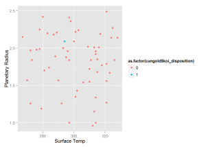
qplot(x = cangold$koi_teq, y = cangold$koi_prad,
      colour = as.factor(cangold$koi_disposition),
      xlab = 'Surface Temp', ylab = 'Planetary Radius')
We see that our model predicts a planet in the "Goldilocks" Zone with probability greater than 0.9. This new planet is potentially habitable for humans beings as it is only roughly twice the size of earth and has an average surface temperature of slightly above freezing. This should be the first planet that NASA attempts to confirm from the "Candidate" list.
Topics from this blog: Student Works