Kaggle: Predicting Allstate Auto Insurance Severity Claims

Introduction

Kaggle competitions are a good place to leverage machine learning in answering a real-world industry-related question. A Kaggle competition consists of open questions presented by companies or research groups, as compared to our prior projects, where we sought out our own datasets and own topics to create a project. We participated in the Allstate Insurance Severity Claims challenge, an open competition that ran from Oct 10 2016 - Dec 12 2016. The goal was to take a dataset of severity claims and predict the loss value of the claim.

EDA and Preliminary Findings

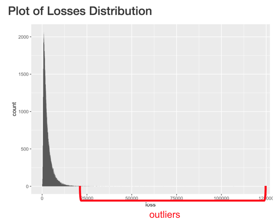
The training dataset consists of approximately 180,000 observations with 132 columns consisting of 116 categorical features, 14 continuous features, and 1 loss value column. The features are anonymized into ‘cat1’-’cat116’ and ‘cont1’-’cont14’, effectively masking interpretation for the dataset and nullifying any industry knowledge advantage. To get a sense of what we are working with, we examined the distribution of the data by building a histogram. It was obvious that the data was very skewed to the right. To normalize the data, we transformed the data by taking the log of the loss.

Since there are so many categorical variables we wanted to find a way to see if we could perform some feature selection. We referred to the Kaggle Forums and saw that we could perform a Factor Analysis for Mixed Data (FAMD). This is sort of a Principal Component Analysis for categorical variables to see if we can reduce our dataset or discover some correlations between variables.

Only 4.08% of the variance in our dataset can be explained from the first five components, which are the highest contributors to the percentage of variance explained. As a result, there is no one particular variable that dominates nor can we reduce our dataset to only a few components. Since there are so many categorical variables, we wanted to find a way to see if we could perform some feature selection. We referred to the Kaggle Forums and saw that we could perform a Factor Analysis for Mixed Data (FAMD). This is sort of a Principal Component Analysis for categorical variables to see if we can reduce our dataset or discover some correlations between variables.

However, a graph of the contributions of the quantitative variables above to the first two components depicts three different groups that may be correlated with each other: a group formed by the upper right quadrant, the lower right quadrant, and the lower left quadrant. Analysis of the categorical variables is not as clear.

Methodology

XGBoost and Neural Networks are known to be strong learners, and we expected them to perform best amongst other machine learning models. However, both as a benchmark and possibility for stacking weak learners, we incorporated other models to compare the cost-complexity and overall performance between them. For the Kaggle combination, the metric is mean absolute error, and we report our cross validation scores and leaderboard scores as such.

Lasso Regression

Lasso (least absolute shrinkage and selection operator) is a regression analysis method, which can perform feature selection and regularization in order to improve the prediction accuracy, providing faster and more cost-effective predictors.

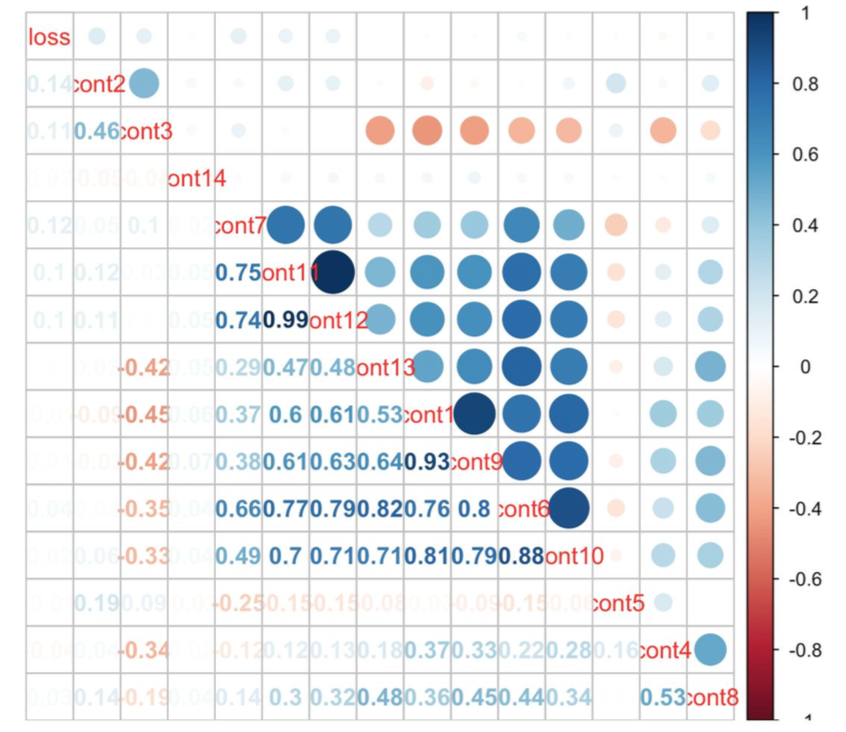
To preprocess the data, we first wanted to remove any highly correlated variables. Looking at a correlation plot of the continuous variables, we saw that variables cont1, cont6, and cont11 were highly correlated with variables cont9, cont10, and cont12 respectively. For the categorical variables, we dummified the variables, converting them from categorical variables to numerical ones. This expanded the dataset’s dimensions from (188318, 127) to (188318, 1088).

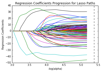
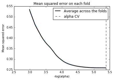
Let’s run the Lasso regression model to explore its ability in loss prediction and feature selection. The training dataset has been split in 80:20 ratio and applied 3--10 cross-validation (5 is ultimately selected) to select the best value of the alpha (regularization parameter). We can see the regression coefficients progression for lasso path in the graph below , which indicates the changing process of coefficients with alpha value.

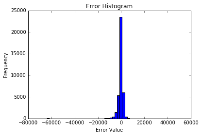
From plots below (“Regression coefficients progression for lasso paths ”, “Mean squared error on each fold”), the best alpha value is 5.377 which could help reduce the number of features in the dummy dataset from 1099 to 326. The error histogram shows the optimized Lasso regression model prediction of the 20% test dataset, the R squared value of this prediction model is 0.56.

Finally, when predicting on the Kaggle test dataset using the Lasso regression model, the prediction results did not rank into top 200 on the Kaggle Leaderboard score. This was not surprising due to a couple of reasons. First, the data does not represent a linear relationship, so the model’s pre-requisites and diagnostics were not good. Also, after the Kaggle test dataset was dummified, we noticed that there were variables that were present in the test set that did not exist in the training set.

K-Nearest Neighbors Regression

We then fit our data using a K-Nearest Neighbors Regression model. The tuning parameter is K, the number of neighbors for each observation to consider. We start with sqrt(N), which was approximately 434 as our initial guess and tune K from 425 to 440.  K = 425 performed the best in this range, though that leaves open the possibility of tuning K in a range around 425. The model gave a CV score of 1721 and a LB score of 1752.

Support Vector Regression

We also used  Support Vector Regression to fit our data . Preliminary cross validation and parameter tuning on our test set revealed that the algorithm was computationally expensive, taking ~12 hours on our machine. Using the sklearn class SVR from the svm module, we attempted to tune cost and epsilon, using a radial kernel and setting gamma to 1/(number of features). Preliminary tuning revealed an epsilon value of ~ 1.035142 , and a cost of 3.1662, giving us a CV performance of 1570. The performance varied greatly amongst the few parameters we chose to test, from 10 to the power of [-1, -0.5, 0, 1] for C and 10 to the power of [0.05, 0.01, 0.015, 0.02, 0.03, 0.1, 0.5] for epsilon for our grid.

Random Forest

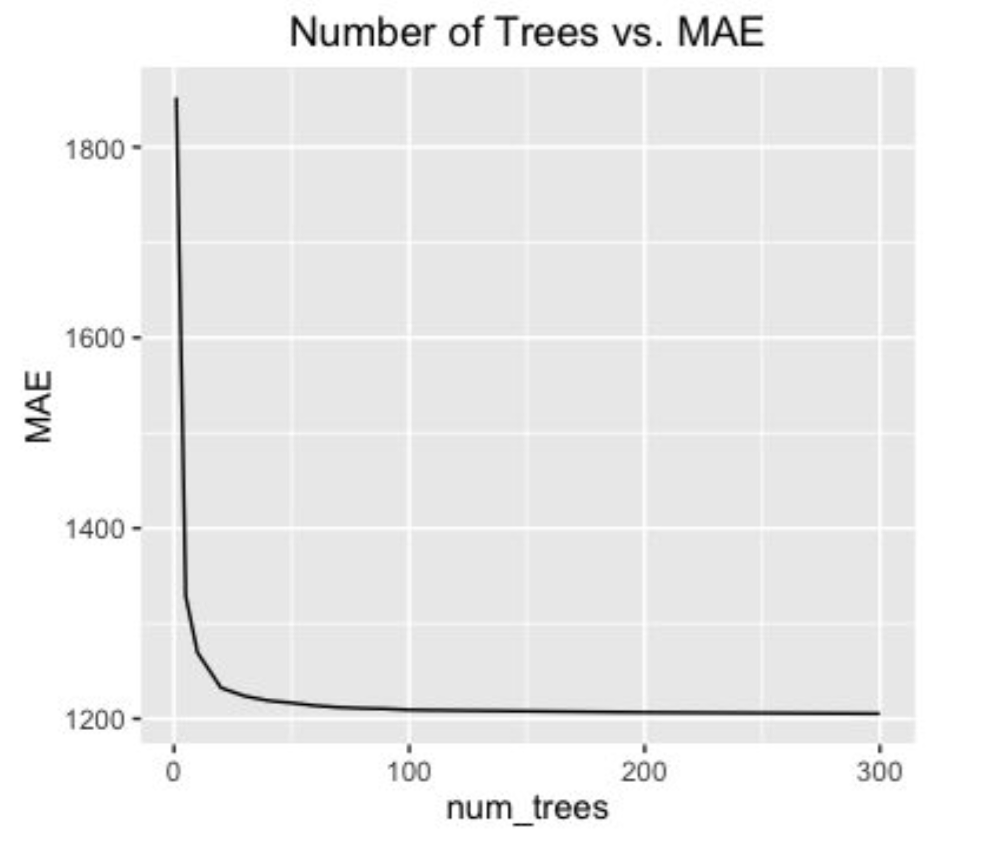
The Random Forest algorithm is a good out-of-the-box model for most datasets since they are quick to train, perform implicit feature selection, and do not overfit to the dataset when adding more trees. For this model, we used the scikit-learn’s package: RandomForestRegressor. To train and validate the random forest model, the data was split using 10-k-fold cross validation. The parameters we tuned were the number of trees and the number of features considered. Initially, the model was trained using all features considered per split. This is essentially equivalent to bagging, which performed poorly, scoring a MAE of 1312 on the leaderboard. To improve on this, we decreased the number of features down to the square root of the number of features. This resulted in the random forest only considering 12 features per split. Using less features forces the model to consider different features per split, which ended up improving the model’s MAE score to 1188.

Training the model on an increasing number of trees improved the predictive power, but took more computational power. To prototype the effects of a model quickly, we used 50 trees to get a sense of the effect and then 200 trees for more computational power. AddIng more trees will help the predictive power, but with decreasing returns. With 200 trees, the best random forest MAE score was 1187. This is the baseline score which we wanted to beat with our more competitive models.

Neural Networks

The Neural Network model turned out to be one of the better performing algorithms. For this competition, we used the Keras (frontend) and Theano (backend) Python packages to build a multi-layered perceptron. Our best Neural Network consisted of three-hidden layers with rectified linear unit activation.

Additionally, we added in dropout and batch normalization as methods to regularized the network. The model was then run with a 10 k-fold cross validation and 10 bagged runs per fold to essentially produce an output that is the average of 100 different runs to minimize model bias. One downside of Neural Networks is that it is computationally expensive. It requires computing many large matrix-vector operations. With an Nvidia GTX 1070 GPU, our model required 5 hours to train. Furthermore, when we tried to add layers or more neurons, the model started to overfit. The model resulted in an average validation mean absolute error of 1134 and a leadership board score of 1113 that put us in the top 25%.

eXtreme Gradient Boosting (XGBoost)

One of the most popular algorithms currently among Kagglers that proved to be successful is XGBoost. This algorithm takes a linearized version of gradient boosting that allows it to be highly parallelized and computed quickly. This allows large number of trees to be produced per model. We chose a learning rate of 0.01, with a learning rate decay of 0.9995. This model also used an average of 10 fold cross-validation with a maximum of 10,000 trees, stopping when the validation error is minimized. The XGBoost model proved to be our single best performing model with a validation score of 1132 and a leadership board score of 1112.

Outlier Analysis

In the Allstate insurance dataset, the data was highly skewed right, with outliers taking on large values. Looking at our validation predictions against the true values, the largest errors accumulate around the outlier points. For this reason, we wanted to see how well we can classify if an observation was an outlier. We chose the threshold that separates an outlier to be two standard deviations above the average loss value. Although the outlier region only made up 2.5% of the data, it made up more than 90% of the range of values.

We first tried to use a logistic regression classifier to establish a baseline. This model resulted in a 97.5% accuracy, which sounds good at first until we realized that this is only as good as the model guessing that all observations were non-outliers. Next we tried a more advanced model, the XGboost classifier with AUC score as the metric to maximize. However when we looked at the output predictions, the probabilities were very close to 0.5 for all observations, which told us that the model could not confidently distinguish the two classes. Also, the AUC score was 0.6 which was much less than desired.

The way this problem was set up, it turns out to be an imbalanced dataset problem where the minority class was much smaller compared to the majority class. One traditional method to deal with these type of problems involved oversampling and artificially synthesizing new minority class and undersampling the majority class. Here we used the Imbalanced-Learn Python package to re-adjust our data ratio from 97.5:2.5 to 90:10. Afterwards, we again used XGBoost classifier and achieved much better results. The accuracy was raised to 99.6% and the AUC increased to 0.80. Although, this was very insightful, this new information did not help our regression model much, so we turned our attention to other methods raise improve our error rates.

Ensembling

Ensembling is an advanced method that combine multiple models to ultimately form an better model than any single model. The idea is that each model theoretically makes its own errors independent of other types of models. By combining the results from different models, we can “average” out the errors to improve our score and reduce variance in our error distribution. For this competition, we chose to do three different ensembling methods with two XGBoost and Neural Network models:

1. Simple average of the test results.

2. Use an optimizer to minimize error of model validation predictions against true values.

3. Weighted average of test results.

First, the simple average resulted in a leadership board score of 1108 already much better than our single best model. Second, the optimizing method resulted in a leadership board score of 1105, even lower than the first score. Lastly, we chose to weigh the better scoring XGBoost and Neural Network heavier with 40% weight each, and the remaining two with 10% weight to sum to a total of 100%. The intuition there was to having the very different models cancel out each other’s errors, while focusing more on the higher scoring models. This resulted in our best leadership board score of 1101.

Results and Retrospective on the Kaggle

With our best scoring model with a MAE of 1101, we were placed at the top 2% of the leaderboard by the end of the two weeks. XGBoost lived up to its reputation as a competitive model for Kaggle competitions, but could only bring us so far. Only after we applied neural network models as well as the method of ensembling, we were able to get to the top 2%.

While trying to perform competitively in the Kaggle was tough. The two week time limit for this project in the bootcamp definitely amplified the difficulty. In order to perform effectively, we needed to have good communication and a good pipeline for testing each model, especially since some models took hours to train. It took a while for the team to build this communication and pipeline up, but eventually we were able to share knowledge and get multiple workflows running.

Although the Kaggle competition was a great way to test our mettle against other competitors using a real-world dataset, there were some detractions in this format. By having a dataset given to us in a clean format, the process of taking data and churning out predictions was accelerated greatly. Moreover, we lost out on attempting to interpret our dataset due to the anonymity of the variables. However, this did allow us to focus on practicing fitting and training models — a huge plus given our limited time. In the future, we would like to incorporate the method of stacking models to see if we could improve our score even further. In addition, we would like to explore other ways in handling the problems with our uneven dataset using methods like anomaly detection algorithms rather than binary classification methods.