Network Intrusion Detection

Project initiated by Joseph Wang and contributed equally by Wanda Wang, Joseph Wang, Radhey Shyam, and Ho Fai Wong. They graduated from the NYC Data Science Academy 12 week full-time Data Science Bootcamp program that took place between April 11th to July 1st, 2016. This post was based on their fifth and final class project - the Machine Learning Capstone project.

I. Introduction

Most businesses, government organizations, and academic institutions house dedicated network security teams which help defend the integrity of internal data or client-facing sites against advanced threats or intrusion attacks. Even at home, you may have a firewall to protect your personal network from outside hackers or attacks. However, as we see on the news quite often, even the most sophisticated organizations and individuals often will have their reputable websites or twitter account passwords compromised.

Recognizing this challenge, our Capstone project focused on developing machine learning (ML) algorithms to tackle detecting network intrusions. We also placed emphasis on balancing model accuracy with interpretability and computational resources at our disposal.

The network connection data in public domains are very limited. The famous data are originated from MIT's Lincoln Lab - which set up a simulated environment to study intrusion detection. This dataset is then used for the Third International Knowledge Discovery and Data Mining Tools Competition that was held in conjunction with the Fifth International Conference on Knowledge Discovery and Data Mining (KDD-99). Later, researchers found there were problems in the KDD-99 dataset as mentioned in the reference. In the capstone project, we used the improved NSL-KDD dataset, which contains 4 main categories of attacks in a local-area network:

• DOS - Denial of service attacks which overwhelm the victim host with a huge number of requests, shutting down a website completely. A famous example you may have heard about was back in 2011 was when the hacktivist group Anonymous crashed PayPal with a DDOS attack after the company refused to process credit card transactions to fund WikiLeaks, costing PayPal lost business.
• R2L - Remote to Local where a hacker attempts to get local user privileges.
• U2R - Hacker operates as a normal user and abuses vulnerabilities in the system.
• Probing - Hacker scans the machine to determine vulnerabilities that may later be exploited so as to compromise the system.

II. Data Exploration

About the data

Data size:

• 41 features
• 125,973 connections in Train
• 22,543 connections in Test

Connection types:

• Train data has 46.5% malicious connections (i.e. attacks) and 53.5% normal connections.
• We wish to classify connections as normal (0) or abnormal (1), and not specific attack types.

Features summary:

• 6 Binary (e.g. is_host_login)
• 3 Nominal/Character (protocol_type, service, flag)
• 32 Continuous

High level categories of variables:

• Basic features of individual TCP connections
• Content features within a connection suggested by domain knowledge
• Traffic features computed using a two-second time window

Initial Exploratory Data Analysis (EDA)

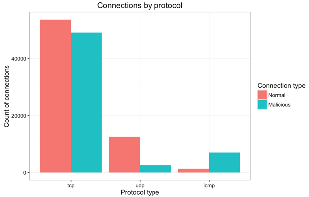
This project would require some basic knowledge of network protocols. We assume that the reader has some basic knowledge of network communications; if not, the internet is plentiful with materials on network protocols and connection flags. Let's start with some initial data exploration on the character categorical features. The bar plot below shows connection type (normal or malicious) by internet protocol (TCP, UDP or ICMP) within the training dataset.

• Most connections use TCP, understandably (e.g. HTTP, SMTP, FTP, telnet, etc rely on TCP); of those, normal and malicious are in almost equal proportion.
• UDP connections are primarily non-malicious (e.g. DNS, DHCP).
• ICMP connections are primarily malicious (e.g. ping and traceroute), used often in DOS attacks.

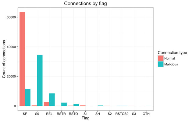
The bar plot below shows connection type (normal or malicious) by TCP connection flag within the training dataset. Each connection has an associated flag indicating the status of the connection e.g. initiated but not acknowledged, rejected, reset, completed successfully, etc. For more details, please read this article.

• Most connections have an SF flag, indicating normal SYN/FIN completion, hence the majority of those are non-malicious connections.
• The large majority of S0 connections are malicious, which makes sense since this flag refers to an initial SYN seen but no reply sent.
• REJ and RST connections (i.e. rejected or reset), though smaller in number, mostly correspond to malicious connections which makes intuitive sense.

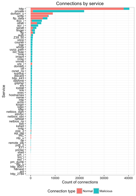
Beyond simply the communication protocols and connection flags, the dataset had a categorical variable with ~70 levels for the service used/requested in the connection.

• HTTP connections are by far the most numerous and non-malicious for the most part.
• Private connections, on the other hand, are primarily malicious in nature.
• SMTP (email) and FTP (data transfer), like HTTP, are mostly used for normal connections.
• There's a long tail of services that are used for malicious connections, though much smaller in overall connection count. However, not all of the low-count connections are malicious (e.g. ntp, x11).

PCA on continuous variables

Given the 32 continuous variables in the dataset, let's run Principal Component Analysis to explore the correlation relationships between variables in the original feature space. The variables factor map below shows the continuous variables projected on the first 2 principal components (which cover 20.56% and 15.04% of the overall variance respectively). We can see groupings of features as described in the graph below, which seem to indicate relationships between predictors that our model will have to streamline. It seems that the first principal component is related to TCP SYN errors while the second is related to TCP REJ errors.

III. Predictive Modeling

Now that we have a better understanding of the features in our dataset.  Let us attempt some predictive modeling to classify connections as malicious (1) or normal (0).

Logistic Regression with Lasso penalty

We trained a logistic regression model with Lasso penalty, to reduce the dimensions in our model for simplicity, and to avoid overfitting while keeping dimensions from the original feature space for interpretability. We split the training set 70%/30% and applied 10-fold cross-validation to select the best value of lambda (regularization parameter). The value of the regularization parameter, lambda, that would have minimized the misclassification error actually retains 110 features, so instead we opted for lambda = exp(-3) which retains 12 features.

Similarly, the graph below shows the trade-off between model complexity (number of features) and overall accuracy. Note the drop in test accuracy with high number of features, as the model is overfitting to the training dataset. However, the most alarming finding is the very large difference between train and test accuracy!

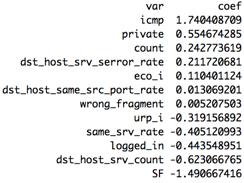
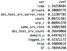
Let's inspect the selected features to see if they make sense. ICMP and private have the highest positive coefficients i.e. are indicative of malicious connections, which aligns with our observations from the basic EDA. Similarly, the connection flag SF (normal connection completion) has the lowest negative coefficient indicating non-malicious connections.

The selected features make sense, so why is there a difference of accuracy from 95% in train to 70% in test? Notably, the test true positive rate is very low at 48% while the false positive rate is actually rather decent at 1.9%. Our test dataset actually also contained response labels, so we wanted to see what would happen if we recreated a train and test dataset by combining, re-sampling and re-splitting the original data into the same proportions. We re-ran the same approach, this time selecting 11 features for the same value of lambda. The test accuracy is now much more in line with the train accuracy: 85.63% accuracy in test vs 91.72% in train!! Also note the decrease in accuracy with higher number of features as we start overfitting to train.

Looking at the selected features and their coefficients again, we notice most of them are similar to the previous model run on unshuffled data.

The true positive rate increased to 72.83% and the false positive rate increased slightly to 2.43% after shuffling our data. Was there some underlying bias in our original test dataset?

Train vs Test Data

We went back to the original data containing the attack types (which we had transformed initially to binary 0/1 for normal/malicious connections). Upon comparing attacks in train vs test dataset, we identified that the distribution of attacks differed:

• 2 attacks in train are not in test.
• 17 attacks in test are not in train.
• Attacks in both train and test could have very different distributions.

Essentially, for this exercise to be realistic, the test dataset needs to contain new attack types that are not present in the training dataset, to mimic a real-world scenario where attackers innovate intrusion tactics and develop new attack patterns to circumvent network security. Shuffling the dataset prior to training our models is therefore a fundamentally flawed approach in this context, so we stuck with the original, unshuffled data instead.

Random Forest

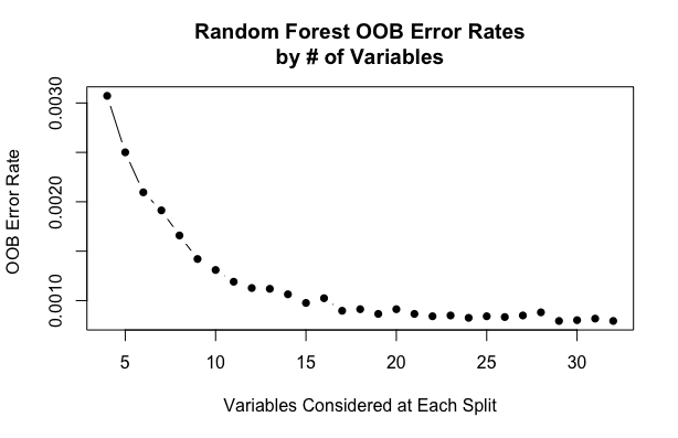
After training logistic regression models, we thought of trying Random Forest. Random Forest model takes  advantage of bagging process where we take different training samples with replacement in order to get predictions for each observation and then average all predictions (or take the majority vote) to obtain the out-of-bag (OOB) estimation.  We predicted the response for the observations which were kept out bag and averaged predictions are used to calculate the out of bag error estimate. For selecting the number of predictors (m_try), we tested for range of predictors and plot the out of bag error vs Variables selected at each split. Finally we selected m_try to be 15 evaluating simplicity and errors.

We set other parameters to default and train the model on the original (unshuffled) data and predicted the responses on unshuffled test data and got test accuracy of 77.21 %, true positive rate, 61.97% and false positive rate, 2.66%. Also, we thought of checking the variable importance plot. The two variables src_bytes (number of bytes from source to destination) , dst_bytes (number of bytes from destination to source) on the top whose coefficients were not significant in Logistic regression.

Next we tried XgBoost (Extreme Gradient Boosting) which  is an efficient implementation of gradient boosting. It is based on the paper "Reliable Large-scale Tree Boosting System" by Tianqi Chen and its R' package "xgboost" written in C++ by  Tianqui  Chen. It has been recently widely used in many machine learning competitions. We find the best learning rate (eta=0.02) from two fold cross-validation and set other parameters to default and train the model on the original (unshuffled) data and got accuracy of 76.94% , true positive rate, 61.57% and false positive rate, 2.75% on the original test data.

Model Comparison

Here we summarize the performance of the conventional machine learning algorithms we employed so far, including Logistic regression, Logistic regression with Lasso regularization, random forest, random forest with Xgboost and Adaboost, and Naive Bayes. As we can see, all the algorithms perform poorly in overall accuracy predictions as shown by the blue bars (less than 80%). The predicted true positive rate (TPR) is extremely poor for the algorithms except the Naive Bayes.  However, the Naive Bayes is the poor performer with high false positive rate (FPR).

 

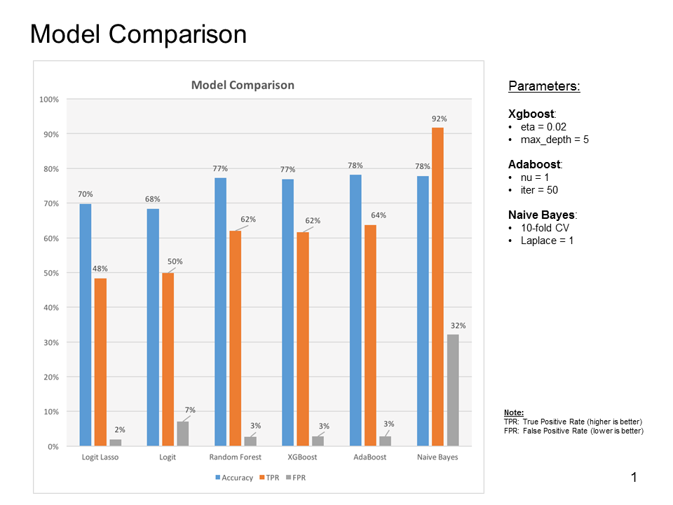
TPR= (#Predicted to be abnormal and actually is)/(#Actually abnormal). FPR=(#Predicted to be abnormal and actually is not)/(#Actually normal).

Principal Component Classifier (PCC)

Based on the network connection data, the conventional machine learning algorithms fail to reach the prediction accuracy even up to 80 percent not to mention the poor true positive (predict to be abnormal and actually it is true) rate as demonstrated in the last paragraph. This implied that we should try a qualitatively different approach to our data modeling. We implemented numerically a novel approach for anomaly detection based on the publication entitled as “A Novel Anomaly Detection Scheme Based on Principal Component Classifier NRL Release Number 03-1221.1-2312”.  The advantage of this approach is to be able to learn the correlation of features which have not been shown in training data. This is particularly relevant for constant evolving malicious attacks from hackers. In addition, PCC is a supervised machine learning algorithm which extends the unsupervised principal component analysis to the domain of the supervised learning.

 

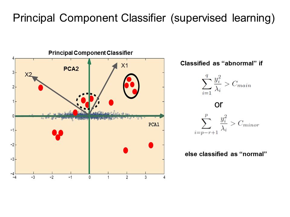
The figure is used for the illustration for the basic idea behind principal component classifier (PCC). The blue open circles are the normal connection records in feature space. PCA1 and PCA2  are the orientations along the main variance and  minor variance direction by the analysis of the principal component analysis for the normal connection data. The red bubbles are the connections which need to be classified as normal or abnormal. For instance,  the connections inside the dashed circle and solid circle, they are all abnormal with very different correlations from normal ones. Cmain and Cmin are the cutoffs for the classifier. yi components represent the principal components along the main variance orientation or minor variance direction in feature space for connection records. The mathematical expressions on the right panels are the distance metrics projected along the main and minor principal directions based on the correlation matrix from the normal connections.

Let us illustrate the idea based on the features in two dimensions first. Imagine we know all the normal connection records (in blue open circles) where we can learn the correlation between features for normal connection through principle component analysis.  The largest variance for the normal connection features points along the PCA1 direction.  However, the PCA2 direction corresponds to the direction with the smallest variance for the normal connections. If there are connections that are very far away from the main distribution of the blue circles, we can classify these new connections as outliers which are malicious in the context. There are two distance measures to characterize the distance. One corresponds to the distance along the small variance direction and the other is along the main principle component. The cutoff for these distances needs to be learned from the training data. To generalize to higher dimensions, both the first few q main principal components need to be considered and the last few r minor principal components need to be considered. Here we selected the first q=4 principal components which account for fifty percent of the accumulated variance and the last p=27 principle components which account for twenty percent of the accumulated variance.

To train the PCC algorithms, we tune the cutoffs separately in the training set to obtain the optimal prediction accuracy for both normal and abnormal connections.  The prediction accuracy is 80%, TPR is 92%, and FPR is 29% lower than that by Naive Bayes. Note that only continuous predictor variables are used as inputs in PCC. We suspected that we can improve the prediction even more if we incorporated the information contained in categorical predictors. To do so, we used the probability outputs from the poor performer, logistic regression without regularization, to ensure all the continuous variables are all considered as PCC. The overall prediction accuracy is up to 83%. The TPR is still comparable. However, the FPR has greatly reduced to 13%. It is a promising strategy to improve the network intrusion detection by stacking PCC with the other conventional machine learning algorithm which can treat the categorical features properly.

IV. Conclusion

To conclude, we have employed machine learning algorithms to predict abnormal attacks based on the improved KDD-99 data set. This data set put a serious test on the conventional machine learning algorithms to be trained to learn very well on training data. Network attacks usually evolve with time and the attack types may not appear in the training. Basic PCC and naive Bayes models outperform others used in this analysis when new attack patterns are not present in the training dataset. To compensate for the missing information from categorical variables, we use the principal component classifier in conjunction with poorly performed logistic regression. We observe a large improvement in our prediction.

Further development of PCC and naive Bayes models could lead to even better model performance for anomaly detection, as well as fine tuning of the poor performed algorithms toward underfitting regimes. For PCC, one can set up the algorithms to learn separately in terms of different categorical predictors or use Support Vector Machine in the principal component space derived from normal connections for anomaly detection. PS: The data exploration and machine learning was performed in R and Python. All the codes are available here.