Zillow Prize: Competing to Improve the Zestimate

Introduction

Zillow is a popular online real estate and rental marketplace dedicated to providing customers with data to make the best possible housing decision. In the “Zillow Prize” Kaggle competition, Zillow released data (3 million observations) with the hope that competitors could use it to help improve the accuracy of the Zestimate, their house pricing algorithm. Our objective was more complex and indirect than simply predicting housing prices from given data though: we were instructed to predict the log errors in the Zestimate, defined as log(Zestimate)-log(Sale Price). Although the Zestimate already predicts house prices within 5% accuracy, machine learning models that closely predict the log errors of the Zestimate would allow Zillow to improve their algorithm further in the situations where it over and under-estimates.

Data Overview and EDA

The first challenge we faced in the Zillow competition was the cleaning and management of the data. We were provided data on 58 features associated with each property. Many of the variables were completely or partially redundant, and over 50% of them had some degree of missingness, sometimes over 97%. Our most fundamental decisions involved which variables to drop and how to interpret existing missingness.

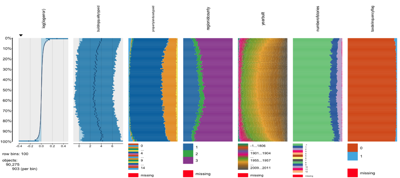
In order to understand the fundamental relationships within the data, we created tableplots, in which we could visually inspect relationships of all variables with log error before removing any missingness. The tableplots suggested variables related to property location and tax would be especially important in our models.

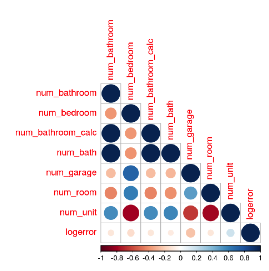
We also created correlation plots in order to understand the pre-existing relationships between variables. Since some machine learning models do not handle multicollinearity well, we eliminated highly redundant variables and used techniques such as PCA and regularization in multiple linear regression to further minimize redundant information.

While modeling, we used an iterative process in which we ran various tree-based models to obtain outputs on variable importance. These results helped us determine which variables could be dropped and which should be kept and imputed in a more sophisticated way.

Missingness and Imputation

The strategy for handling missing data was one of the key challenges of this project.  Our approach to this problem was to systematically assess each variable, in order to better understand the reason for missingness.  These variables can be separated into two broad categories: first, those in which the reason for the NA is implied by the data, and second, those for which the reason for the NA is unknown.  

For several of the variables with high missingness, we believe that missing data points simply implied that the property does not contain the item in question.  These variables contain a distribution of ones, signifying that the property contains the item, intermixed with NAs.  These categories include topics such as tax delinquency, lot size, fireplace, pool, garage, basement, and hot tub; it makes intuitive sense that many of the properties in southern California do not have some or all of these features.  Thus we imputed NAs in these categories with zero to signify that the feature is not present for those observations.  

For other variables, the reason for missing data is less clear.  For features such as unit count, bedroom count, bathroom count, number of stories, or year built, missingness was relatively high and it does not make sense to consider an NA as a feature that is not present for a given observation.  Imputation is more problematic in these cases, as KNN can not be realistically calculated on the full Zillow data set within the time allotted for this project and mean/median imputation can change the distribution of the variable, which could induce further error into the predictions. We also hypothesized that missingness in these variables could help to predict log error in sale price vs. Zillow’s estimate, as it is possible that Zillow has more difficulty predicting value for an observation that is missing more variables.  Thus, for these variables we imputed with -1 to preserve any possible hidden reasons for missingness in these observations.  

We used mean imputation for the calculated finished square feet variable, as this variable is nearly complete, so imputing with the mean value has a negligible effect on the overall distribution of the variable.  We dropped the other floor space variables, as they are either entirely redundant or highly missing.  For the location variables, missingness was also very low, so we imputed by randomly sampling from the distribution of each variable.  

Given the importance of the tax assessment features, we took care to make informed imputations for missing values. For properties with property taxes paid values, we divided these values by the median tax rate (these were fairly consistent) across all properties to get an estimated assessment value. Over 99.9% of these cases had zero bathrooms and zero bedrooms, so we imputed the estimated assessment value as the land assessment, and imputed zero for the building assessment. For properties with no taxes paid values, we imputed the average building and land assessment values, grouped by zip code, number of bedrooms, and number of bathrooms - assuming that properties with the same number of beds/baths in the same zip code were likely to have similar land and building assessment values.

Data Transformation

Since some machine learning models require normally-distributed, scaled data, we transformed certain variables for these cases. Before performing linear regressions with regularization, we were careful to check the distribution of each variable, transform it if necessary, and then scale it. One effective way to do this was to employ a skewness function on each variable:

skew.score <- function(c, x) (skewness(log(x + c)))^2

In this function, c is a constant added to the data before log transformation. Our goal was to find the value of c which gave a skewness value as close to zero as possible. Then, we plotted the data visually to inspect the results of each transformation.

Multiple Linear Regression

The multiple linear regression process was conducted iteratively, starting with selected features that intuitively made sense and subsequently trimming the number of features used. The first linear model tried included variables related to amounts of land and structure taxes paid, whether there had been a tax delinquency in the past, and ones pertaining to the overall structure of the houses (numbers of bathrooms, bedrooms, garages, and types of hot tub or pool, if any). The result was poor, as the R-squared of the model was below 1%, and several features had high VIFs, suggesting multiple instances of multicollinearity. In addition, the QQ-plot and residual plots showed that assumptions underlying linear models were violated, including heteroscedasticity and lack of normality of the residuals.

As several features tried in the first model also had large p-values, the second attempt removed those that had both high VIFs and large p-values. However, the result didn’t yield any improvement, as the R-squared remained under 1%. Although VIFs across the features that remained were within more normal ranges, the model as a whole didn’t provide adequate explanatory power.

Further trimming the model continued to demonstrate promising signs of improvement, which led us to add regularization to the model. Shrinking the coefficients did produce better results, as both ridge and lasso regression models generated MSEs that were both reasonable. The final model picked for presentation included only six features: finished square footage of the property, square footage of lot, tax amounts, number of bedrooms, and number of units. However, since the linear assumptions were still violated, meaning fitting a linear model – however modified – to the data was simply not the best method.

Random Forest

We used grid search and cross validation to optimize our Random Forest model on three key parameters: number of variables considered at each split (mtry), number of trees to grow for each model (ntree), and minimal size of terminal nodes (nodesize).  We left the maximum number of terminal nodes (maxnodes) to grow to the level determined by the nodesize parameter.  We also considered variable importance, by testing versions after eliminating some of the less important variables

Due to the high computational complexity of the random forest model on large data sets, we initially sampled 10-25% of the Zillow data to more efficiently narrow down the search for optimal tuning parameters.  We then used a 75%/25% training/test split on the full data set for precise model tuning.  

The optimal Random Forest model featured mtry = 2, ntree = 1000, nodesize = 12 observations, and included all variables, generating an MAE of 0.0658.  Despite the time invested in cross validating and tuning to arrive at the optimal parameters, this result was outperformed  by several other models (both simple and more complex).  While the result from the standalone Random Forest model was disappointing, this model was useful in determining variable importance to assist in variable selection for other models, and was useful as an input for our final ensemble model.  

Gradient Boosting

Gradient boosted models are ensembles of decision trees, the same fundamental structure used in random forests. Instead of averaging the predictions of hundreds of independent trees, boosting takes an iterative approach - build a tree, calculate the output of your objective function (incorporating training loss and regularization), and use this output as an input for the subsequent tree’s objective function. Boosting adjusts the weights associated with each split in a tree based on the error from the prior tree - slowly descending along the error gradient (gradient descent) until the algorithm can settle on a local minimum that optimizes your objective function. A “learning rate” hyperparameter lets you decide the rate of descent. Some other important hyperparameters are the number of trees, maximum tree depth, and minimum number of observations per leaf.

Gradient boosting performs well for most machine learning problems. One drawback relative to random forests is boosted trees are necessarily dependent, so your model may suffer from overfitting.

This is an oversimplified description of the gradient boosting process. For more info, the creators of XGBoost have an excellent description here.

Analytics Vidhya also has a great tutorial on hyperparameter tuning in gradient boosted models here.

Our team used sklearn’s gradient boosting regressor on a number of numeric and categorical variables, resulting in our most successful model, with a mean absolute test error of .0516. We used 5-fold grid search cross validation to choose hyperparameters.

XGBoost

We also used XGBoost, a package that 1) has computational advantages over sklearn’s gradient boosting (i.e. it runs faster), and 2) includes regularization at each step of the process to control for overfitting. This paper has a great description of XGBoost. Analytics Vidhya’s hyperparameter tuning tutorial here.

Our best XGBoost model, tuned using 5-fold grid search cross validation and using the same features as the sklearn gradient boosted model (GBM), performed slightly worse than the GBM with a mean absolute test error of .0529. As we mentioned before, XGBoost regularizes at each step. Ridge regularization performed better than Lasso or Elasticnet.

While GBM and XGBoost gave us our best performing models, we noticed that both were conservative in their error predictions. The below graph compares actual logerror distribution to the predicted logerror distributions using our best GBM and XGBoost models.

k-Nearest Neighbors (k-NN)

k-NN is another non-parametric regression method we decided to explore. k-NN calculates the “distance” (typically either Euclidean or Manhattan) between each observation based on their features. Observations with smaller distances between them are closer “neighbors”. k-NN takes the k closest neighbors and averages the logerror (or whatever outcome variable) among them as the prediction. k-NN can also compute weighted averages based on distance (i.e. closer neighbors count more).

We thought this algorithm made the most sense given our problem. When people buy and sell houses, they typically look at houses that are most similar (“comps”) to inform pricing. k-NN identifies the k most similar properties and uses only those properties to inform the logerror prediction.

We used 10-fold cross validation to choose the k (the number of neighbors), and landed on 10, right around the elbow of the below graph.

Our initial k-NN model had a fairly low mean absolute test error of .0567, and the distribution of predicted logerror values was more consistent with the actual distribution of logerror values - meaning it didn’t underestimate as badly as the GBM and XGBoost models (see below graph).

However, k-NN scales poorly with more observations and features. When we used this model to predict the values for the entire properties dataset (over 3 million rows), it took over 10 hours and our computers crashed. As a next step, we hope to use dimensionality reduction techniques and a more powerful computer to put this k-NN model into production for the Kaggle competition.

Model Ensembling

With all of these regression models in hand, we ensembled the five highest performing ones - averaging the predicted logerrors of each model to inform the final logerror to submit to Kaggle. The theory behind ensembling is that incorporating the predictions of multiple models results in less biased predictions. You are seeing the problem from different viewpoints and can leverage the strengths of each perspective. Our ensembled predictions performed markedly better on Kaggle than our best single model, the GBM - consistent with our expectations.