Predicting Housing Prices in Ames, Iowa using Advanced Machine Learning Techniques

Introduction:

Buying a house in today’s economy is an expensive proposition. As millennials flee the housing market in search of more affordable living options, realtors and corporations are scrambling to find ways to make properties on the market attractive to what buyers are left. Being able to predict what the housing prices in a particular market might look like in 10 or 20 years would be a particularly valuable practice in this endeavor.

Cue Notorious B.I.Ggplot (Angie Lin, Chris Castano, and Kat Kennovin)! Our group used the dataset listed on the Ames, Iowa, housing data Kaggle competition that was compiled by Dean De Cock to see if we could successfully predict the prices of houses for which we had no sale price.

Provided here is a link to the Github repository for a further detailed review into the code used:

https://github.com/angielin59/projectML

Missing Values and Data Preparation:

Our team decided early on in our process that we wanted to use a tree model to predict the sales prices. However, before we could get started training our model, we needed to deal with the missing values in our dataset. The most common form of “missingness” was the inclusion of the value “NA” in the dataset. This usually means that a value was not recorded. However, the notes for the dataset revealed that this value often denoted instances where there was no relevant information, rather than a value that had been left out of the dataset. For example, if there was a value of “NA” for the variable which recorded the basement area, it meant the house did not have a basement rather than the basement area had not been properly recorded. However, when reading a CSV file into Python, it is set by default to interpret the string “NA” as a true Null value which will interfere with our analysis and prediction models. To rectify this, we filled in a value of 0 where appropriate for numerical variables and values such as “NoBasement” or “NoGarage” where appropriate for categorical variables.

We dummified certain ordinal variables to see if we could extract further information from the values within. For example, “LandSlope” was originally indicated with categories “gentle”, “moderate”, and “steep.” This could be changed to rank the severity of the slope with nominal values, like 0, 1, 2, where 2 is the steepest rank.

For the quantitative variables denoting the year the garage was built and the lot frontage, we imputed the missing values as the mean and median, respectively, of that variable rather than filling in a 0. For year garage was built, we did not want to use a 0 for missing values, even though there was no garage at this house, as this might skew the data in this variable. We filled missing values in this variable with the mean of the total data for year garage was built. It also did not make sense to fill in a 0 for missing values in lot frontage, which is a variable that gives the distance of the street in linear feet which is connected to the front of the house property. For this variable, we were confident a missing value was a true missing value, rather than the house was not touching a street. For these missing values we created 10 equally sized bins to split the data into by lot area. We then used the median of lot frontage in each bin to fill in the missing values that fell within each bin.

We dropped two variables: “PoolQC” and “MiscFeature”, which meant Pool Quality and Miscellaneous Feature respectively. There were so many missing values (each more than 1400 missing values out of 1460 total observations) that we thought if we imputed our own, it would be us telling the dataset about itself, and the not the dataset telling us about itself.

Initially, we actually dummified too many variables. As it turns out, dummifying categorical variables doesn’t help a tree model all that much unless you have more than 50 categorical variables. As we only had 43, we un-dummified the majority of our own which improved our models.

Feature Engineering:

We added several variables to the dataset to see if we could increase the accuracy of our model. Some of them were quantitative variables that made looking at the data easier. Some were categorical variables that we thought off the top of our heads might make a difference. For example, we thought it would be more likely that buyers would purchase homes in the summer since families do not want to move during a school year. We created a column called “seasonality” to take this trend into account, which gave each observation a named season based on which quarter of the year it fell into combined with the year sold (for example “Fall-1992”). On the quantitative side, we did things like adding together all the square footage-related columns in the dataset in order to get the total square footage of the home. Among the new variables we added were “Total Square Footage”, “Seasonality”, “Remodeled”, “New House”, and “Total Bathrooms”.

Later when implementing these variables into our model, if we used some variables to compute a new one, we would run our model with both the old variables and the created variable, and then again with just the newly-created variable to see if it made a difference in terms of accuracy. Sometimes it did, and sometimes it didn’t. Depending on its effect, we would keep or release variables.

Finally, we added a variable consisting of an entirely random vector of numbers. When we analyzed feature importance of our tree models, we could then conclude any variables which performed worse than the random variable were not making a significant contribution to our model. These variables and the random integer variable were then dropped from the dataset.

Random Forest:

After running an initial tree model to see where it is we were starting, our team immediately jumped into using random forests in order to get some information on feature importance. As previously mentioned, one of the variables added was “randInit”, which assigned each observation a random number. Any variables that had less importance than randInit were selected to be dropped from the dataset, as the variables are essentially “worse than random.”

To further determine which variables should be kept, the data was split into a training and test set (80% - 20% divide respectively). We tested which subset of variables gave the lowest test MSE and used that model as the final model to tune and use for a boosted tree model.

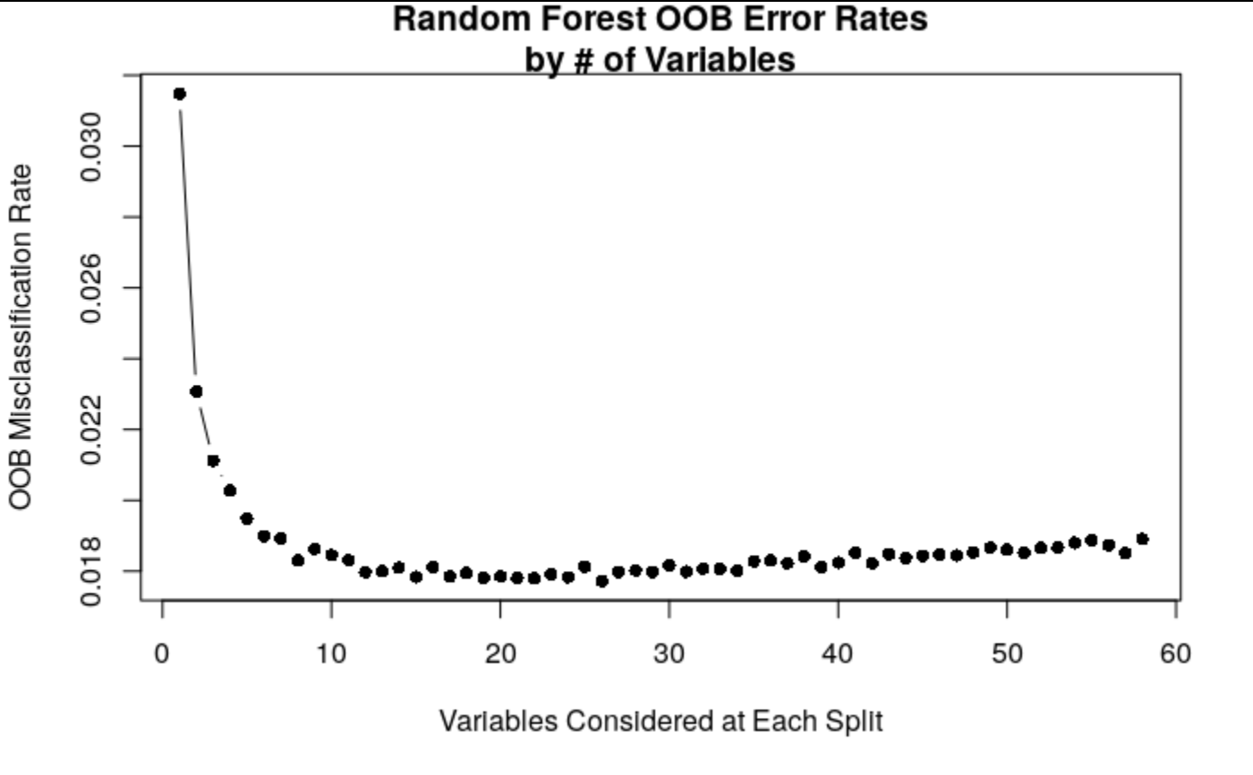
When plotting the Mean Standard Error vs. the number of variables considered at each split of our tree, we found that our “elbow”, or where the error began leveling off, was between 3 and 15 variables. In this range, 15 variables considered at each split provided the lowest MSE. However, running a random forest with 15 variables per split only provided a marginal improvement with a RMSE of 0.14373 compared to an earlier RMSE of 0.14378.  

Boosted Trees:

We then used a boosted tree model to reduce our error even further. Here, our goal was to find which number of trees used in our model would give us the best MSE.

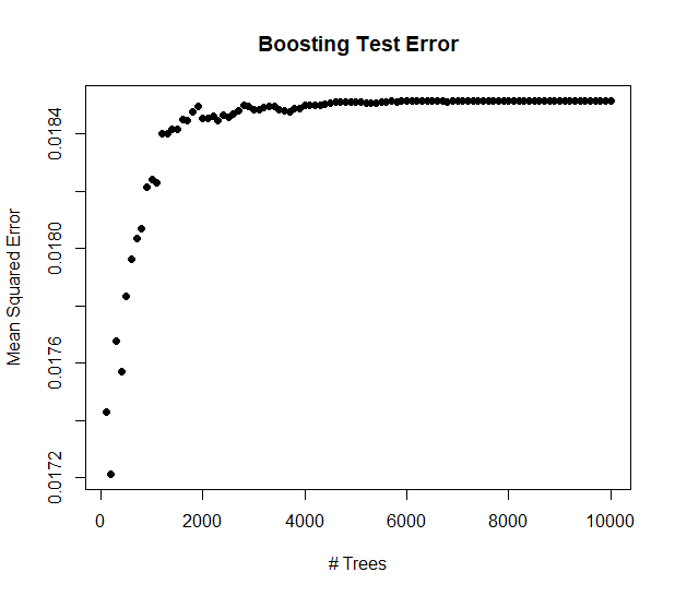
Ultimately, our team determined that while variance decreased as the number of trees increased, the error in our model increased as well. With our final dataset after feature engineering, we found that the optimal number of trees to use in our boosted model was 200. This boosted model would produced our best RMSE of .12514.

Future Work:

There are several areas in which our model could improve.

Given that the boosted model gave our team the best outcome, we would like to spend more time further tuning the hyperparameters other than number of trees used to see if they could give us an even better result. We could potentially tune interaction depth, minimum observations allowed per terminal node, and more.

In the future, we would also like to explore the possibility of stacking our models. Simply taking the average of the predictions from our final random forest model and final boosted trees model produced an RMSE marginally worse than our boosted trees RMSE. However, we think that combining the best predictions of both models would potentially lead to a better result.

Finally, spending more time on feature engineering is always welcome. Given more time, we’d enjoy creating more variables and data subsets to improve our models even further.