
Background
Objective
The goal of this project was to predict real estate market values in Ames, Iowa. We set out to model housing prices based off a wide-range of features categorized in a dataset from kaggle.com. We employed a variety of machine learning models and algorithms to manipulate, train, and fit data for predictive analysis.
Machine Learning
The general process can be visualized below:
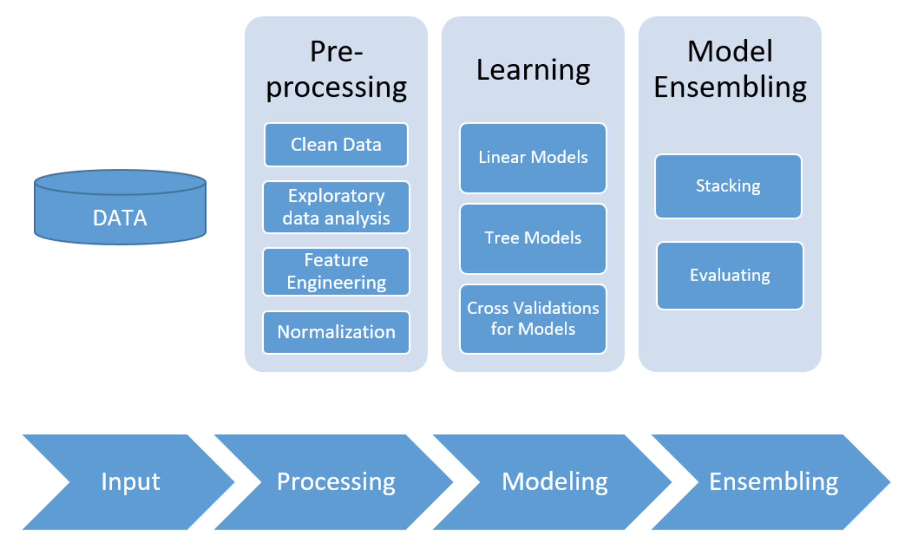
Preprocessing & EDA
Cleaning Data and Exploratory Data Analysis
The raw data had 35 columns with missing values. First, we appropriately imputed missing values, taking into account the information from the data description file. The variables were split into different groups in order to account for each of their specifications.
An abridged snapshot of columns with missing values can be found below:
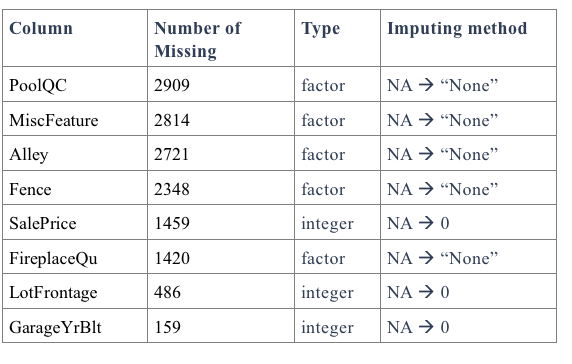
Fourteen of the factor variables (mainly the ones associated with quality and condition) had levels that needed to be assigned. After that, we recombined all the groups as training and testing sets.
Feature Engineering
For feature engineering, we created and adjusted current variables by taking practical business questions about real estate transactions into consideration and came up with the new features described below:
- Total square feet: Sum of general living area square feet and total basement square feet
- Bathroom number: Full bathroom # + 0.5*Half bathroom number for both general living area and basement
- Is New: Check whether Year Sold is the same as Year Built
- Remodeled: Check whether Year Built is the same as Year Remodeled
- House Age: The difference between Year Sold and Year Remodeled/Built
- Total Porch square feet: Add up all porch related square feet
Data Transformation / Normalization
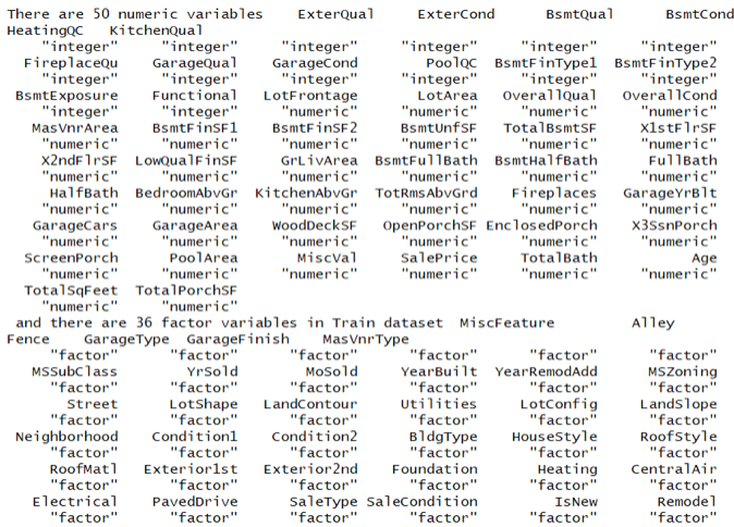
After feature engineering, we had 50 numeric variables and 36 categorical variables.
We applied one-hot encoding methods to the categorical features to “binarize” the category and include it as a feature to train the model.
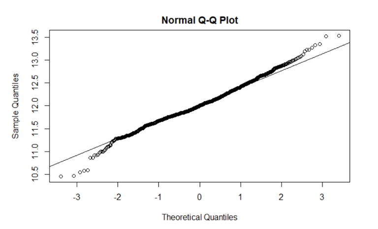
We also checked skewness. For example, the Q-Q plot below shows that sale prices are not normally distributed. We calculated that there is a right skew upward to 1.879.
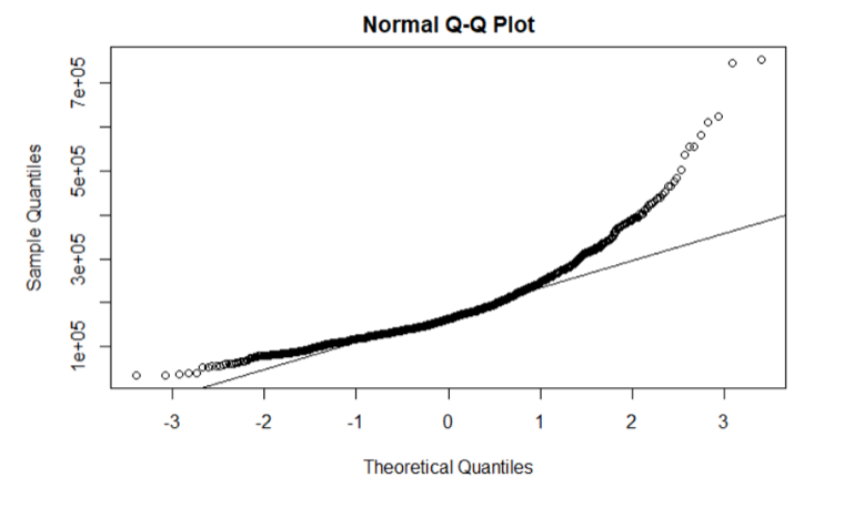
To correct for this, we took the log of SalePrice. By consulting the Q-Q plot below, we found that the transformed sales price is normally distributed.
After correcting for the SalePrice variable, we repeated this process for all remaining numeric variables. We performed log transformation on any variable with a skew larger than 0.8 (normalizing the data with the perProcess function).
Linear Modelling
Modeling
We considered a number of models when building our ensemble. Among them were:
- Linear Models
- Multiple Linear Regression
- Ridge Regression
- Lasso Regression
- ElasticNet Regression
- Tree-based Models
- Bagging
- Random Forest Regression
- Boosted Methods
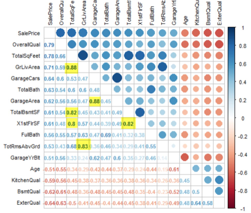
We think these two types of models capture the nuances of the data and produce accurate prediction results. Because some of our predictor variables show strong linear correlations with other predictor variables (as visualized below), we applied several regulation methods.
Hyperparameter Optimization
We applied the conventional 5-fold cross-validation (CV) for both linear methods and tree methods in order to get a more dependable evaluation of our models' functioning. This technique splits the dataset into five-folds. The algorithm is trained on four folds and tested on one; it then repeats this step five times, each time with a different fold acting as a test set. With our CV algorithm, we utilized the "grid search" method in the R caret package, which is designed to make finding optimal parameters for an algorithm very simple. The grid search will execute every combination of parameter values and select the set of parameters highest performing model.
Linear Models: Multiple Linear Regression and Regularized Linear Regressions
The Lasso, Ridge and Elastic Net are regularization algorithms that limit the risk of overfitting by introducing information. These methods introduce a shrinkage penalty fee to a cost function. The estimated coefficients of the predictor variables are shrunken towards zero relative to the least squares estimates.
Ridge regression is similar to residual sum of squares (RSS), but there is a shrinkage penalty (lambda) which acts as a tuning parameter. Its advantage lies in the bias-variance tradeoff made possible by lambda (as lambda increases, bias increases, but variance decreases). It cannot select variables. We can infer which variables are important based on which are further away from zero at lower lambdas, but we cannot select anything at this point.
Lasso regression -- unlike Ridge -- can, in fact, select variables as the Lasso penalty forces some variable coefficients to be exactly zero when lambda is very large. This makes variable selection possible (we drop the variables that are exactly at zero).
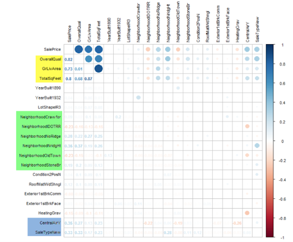
We targeted variables with a lasso importance score higher than 0.05 and plotted the correlation with sales price.
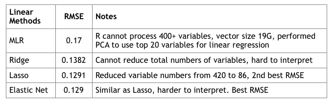
Elastic Net linearly combines penalties from Lasso and Ridge and enjoys benefits from both methods. As we can see from the table below, regularized models enjoy lower RMSE values than general multiple linear regression without regularization.
Tree - Based Modeling

While Decision Trees are not always an optimal approach, they can be useful for their interpretability. By aggregating different approaches, we were able to improve our model’s accuracy.
Bagging
First, we tried bagging. Bagging generates many copies of the original training data set using the bootstrap, fits a separate decision tree to each copy, and finally aggregates all of the trees in order to produce one model.
Conceptually, we realize that bagging can lead to high variance and overfitting. Most or all trees in a “bagging” scenario would include a strong predictor in the top split, leaving all the bagged trees looking similar to one another. Consequently, the predictions from the bagged trees would be highly correlated.
Random Forests
In order to limit the risk of overfitting, we implemented a random forest algorithm over the bagging in order to de-correlate the trees. We randomly divided observations into test and training sets and applied random forests on the training set for different values of the number of splitting variables. For this model, this means that each time a split in the tree occurs, a fresh set of predictors is considered. Therefore, in random forests, at each split in the tree, the algorithm is not even allowed to consider a majority of the available predictors. This forces the algorithm to have many tree splits that do not even consider a strong predictor (a predictor that is highly correlated to others) .
After averaging over a collection of de-correlated trees, our model yielded a RMSE of 0.1562. With the de-correlative effect of random forests and with a big enough number of trees, we do not have to be concerned with overfitting.
Boosting
In the boosting algorithm, trees are grown sequentially: each tree grown based on information from previously grown trees. In implementing this model, we had to take into account the fact that if the the number of trees is too large, a boosting model can lead to overfitting. We used fold cross validation to find the best hyperparameter values and established that the number of splits in each tree (a.k.a. "depth”) should be four.
In our R code, invoked the XGBoost software library that provides a framework for gradient boosting. It is known for its high accuracy, scalability, and speed. Through this method, we achieved an even lower RMSE of 0.1294.
Conclusions

Ensemble Methods
We decided to take a weighted average of our Elastic Net regularization linear model and Boosted decision-tree test predictions. Elastic Net linearly combines the penalties of the lasso and ridge regularization methods, thereby solving the limitations of both methods. Elastic Net models allow for feature selection even in the presence of multicollinearity among the predictor variables.
At every step, we had to weigh the benefits of bias minimization against the associated costs and risks of overfitting. This was no different when finalizing our model; we always have to consider the Bias-Variance tradeoff. If the models we stacked were too similar, we could risk overfitting. Hence, we decided to bridge the various techniques we used. We combined Elastic Net regularization and Boosted decision-tree test predictions according a weighted average. Stacking a diverse ensemble of algorithms boosted our model's predictive accuracy.
Sources:
An Introduction To Statistical Learning with Applications in R
Gareth James-Daniela Witten-Trevor Hastie-Robert Tibshirani - Springer - 2017
Link to Github and Source code:
https://github.com/mwp42/Machine_Learning_Project
https://gist.github.com/mwp42/6f8fc34695e5c517dfc380d51aff87b1
Topics from this blog: R Machine Learning R Visualization Student Works