Higgs Boson Machine Learning Challenge

Contributed by by Belinda Kanpetch, Taraqur Rahman, Steven Ginzberg and Michael Winfield.  They are currently in the NYC Data Science Academy 12 week full time Data Science Bootcamp program taking place between January 11th to April 1st, 2016. This post is based on their fourth class project - Machine learning(due on the 8th week of the program).

Introduction

The Higgs Boson Challenge, hosted by Kaggle, asked the data scientist community to utilize machine learning to accurately predict if a particle was a Higgs-Boson particle or not; more specifically if a signal detected was either a ‘tau tau decay of a Higgs boson’ or just ‘background’.

The datasets provided were the training and test set with 250,000 and 550,000 observations, respectively. The training set contained all the same features as the test with two additional columns of ‘Label’ and ‘Weight’ that gave the accurate classifiers to help train our models.

Our approach for this project was to get a little background on the physics and cursory understanding of how the experiment was performed.  We looked at correlations between the variables and noticed that a few were highly correlated and thus began researching how other scientists had suggested working with the correlated variables.  This lead us to the feature engineering discussed below. In addition, we all utilized the Caret package in R for all coding.

Check out our github to see the code.

The sections below will unpack:

• How we approached missing values
• Feature engineering
• XGBoost model
• Gradient Boosting model
• Random Forests
• Neural Networks
• Conclusion & Next steps

Missingness & Feature Engineering

The missing values in the dataset (-999) resulted from two sources:

1. Bad estimates of the mass of Higgs boson; and
2. Jets: particles that can appear 0, 1, 2, or 3 times in an event.

To deal with this structural missingness, we:

• Converted the -999s into NAs.
• Created a Boolean column to reflect missing(T)/present(F) values in the estimated mass of the Higgs boson (DER_mass_MMC).
• Created 8 binary columns reflecting each combination of presence(0)/absence(1) in the estimated mass of the Higgs boson and the number of jets (0,1,2,3).
• o J0 +M1, J0+M0, J1+M1, J1+M0…
• Imputed the column mean for all the NAs.

For more on the structural nature of the missing values in the Higgs boson dataset, see cowa14.pdf.

Feature Selection

To deal with the risk of overfitting, we:

• Subtracted the PRI_tau_phi column from the other 4 ‘phi’ columns.
• Rotated the angle of the remaining 4 phi columns.
• Deleted all 5 of the non-rotated phi columns, leaving us with 4 phi columns instead of 5.

This subtraction + rotation process makes the specific pattern of the phi variables more unique, so that, once the model is trained, it is better able to discriminate between signal and background in the test set.

For more on the logic of this process, see diaz14.pdf

XGBoost

Our team explored XGBoost for a few reasons. First, it ran relatively quickly; and second there seemed to be a fair number of tuning parameters available to play with.
Playing with the model and actually getting it to a good fit are two completely different concepts.  In general, we split the training set: 80% of the training set to train the model, and the remaining 20% as a test set.  In all cases we used the AMS as the deciding metric, and measured accuracy as the percentage of the 20% test data correctly ID’d as our  performance indicator.
Some of the tuning parameters used were:
•    Number of cross-validation folds, between 2 and 5
•    Number of rounds, between 50 and 400
•    Eta (shrinkage) between .001 and .6
•    Gamma between .01 and .6
•    Max tree depth between 6 and 10
Generally, we received AMS scores on the training (80%) set of between 1.2 all the way up to 1.8+.  These resulted in accuracy rates of 80%+ when applied to the test (20%) dataset.  Our first instinct is this was overfitting, and that turned out to be the case.  The AMS scores on the Kaggle full test data site were much lower, with the highest being about .5.

Gradient Boosting Model

We implemented a GBM to compare with the other non-linear models performance.  Our intuition was that this would be a good comparison with the Random Forest since they are both tree based methods but are grown in different ways; with GBM taking into account the mistakes or residuals of the previous trees. We had to be cognizant of overfitting and adjusting parameters to make the learn the model slowly.

The train.csv file we received from Kaggle was split into an 80% train and 20% test sets. Using the Caret package we implemented an expanded grid of parameters to train the model.

https://gist.github.com/bkanpetch/58729cdc674bad93adb7d3c5ff027c51

This returned an optimal model with parameters and score below.

Although the accuracy was better than a 50/50 chance it did not perform as well as we had anticipated. Therefore, we trained another model with a larger number of trees and larger lambda, or shrinkage, to try have the tree learn slower.

https://gist.github.com/bkanpetch/35c520d8880916774b954dc4803667be

Of the parameters we specified, an optimal model with parameters and score were returned below.

It is interesting to note that even though the second model returned a lower accuracy rate the Kaggle score was higher most likely due to overfitting.

Some challenges were the lack of computational power as we very soon learned that running GBM was computational expensive and took hours to train one model.  Additionally, in hindsight we should have started running a substantially larger number of trees.

Random Forest

For our RF model, we tried both bagging (mtry=38) and a number of other mtry values (7, 12, 38).  We trained on the entire training dataset and used the out of bag error instead of cross-validating with 80% of the dataset.

Overfitting due to leakage was not an issue with the model due to the feature engineering on the dataset that substantially reduced its multicollinearity.

Using parallel processing and a server enabled this model to run well in under 3 hours.

In hindsight, we could have used the number of trees for the RF model as a benchmark for determining the point at which a boosted trees model outperforms the RF, rather than allowing the Caret package to select the optimal number of trees itself.

Neural Network

We applied the neural networks to our dataset that we feature engineered. We believed the weight decay was crucial for the neural network. The weight decay is a multiplier that determines the significance of each node in the network. If it is extremely small then that means that node has no effect on the output. If it were big then the node would have a significant impact on the output. During the process of neural networks, each input goes through a node. When there are multiple nodes, one way the network knows which node to take precedent is by assigning a “weight” or value to it depending on how significant that node is for the prediction. The weight decay is a useful multiplier that neural networks use to automatically go backwards to adjust the weights if they are not that significant in coming up with a prediction.

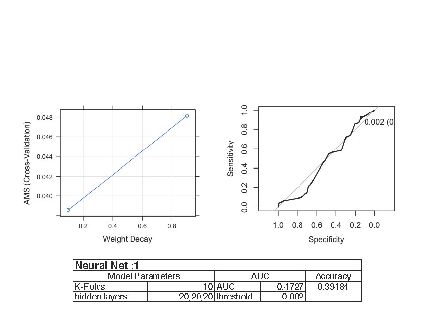
For the first neural network trial, we tried to implement three hidden layers of twenty nodes each. Our understanding was that since weight decay is applied, we would not have to worry about overfitting. However we were wrong. This model produced a threshold of 0.002 (graph of Specificity vs. Sensitivity). Specificity is the false negatives while the Sensitivity is the true positives. The maximum point where the sensitivity and specificity were optimal was at 0.002 (threshold).

Learning from our mistake, we chose different hidden layers since even with the weight decay, overfitting is possible. This time we used one hidden layer with 20 nodes. This produced a better threshold of 0.041 and a better accuracy.

During our research we came across another neural technique called dropout neural network. Based on our understanding, in an ideal scenario, neural networks would like to go through each node and see what its exact weight would be and average all of them. However it is computationally expensive. The way the dropout method works is that it randomly “drops” a node and then calculate the weight of the others. Once it gets to the end, it will go backwards and drop another node and adjust the weights accordingly. With this technique, there are fewer nodes to calculate and therefore it would be close to the ideal scenario without the expensive computations. This works because all the nodes have a fifty percent chance of dropping which prevents the technique from being bias. We believed this would be great to calculate for the AMS.

Conclusions and Next Steps

What we would like to do next:

• Look into ensembling models
• Exploration of other packages other than Caret.
• With more time, we could have written a function that:
  • Identifies values of PRI_tau_eta < 0
  • Converts the signs of all eta values in the same row (- to +, + to -)
  • Imputes the column mean for missing values and randomly assigns a sign (+,-)
• http://www.jmlr.org/proceedings/papers/v42/diaz14.pdf

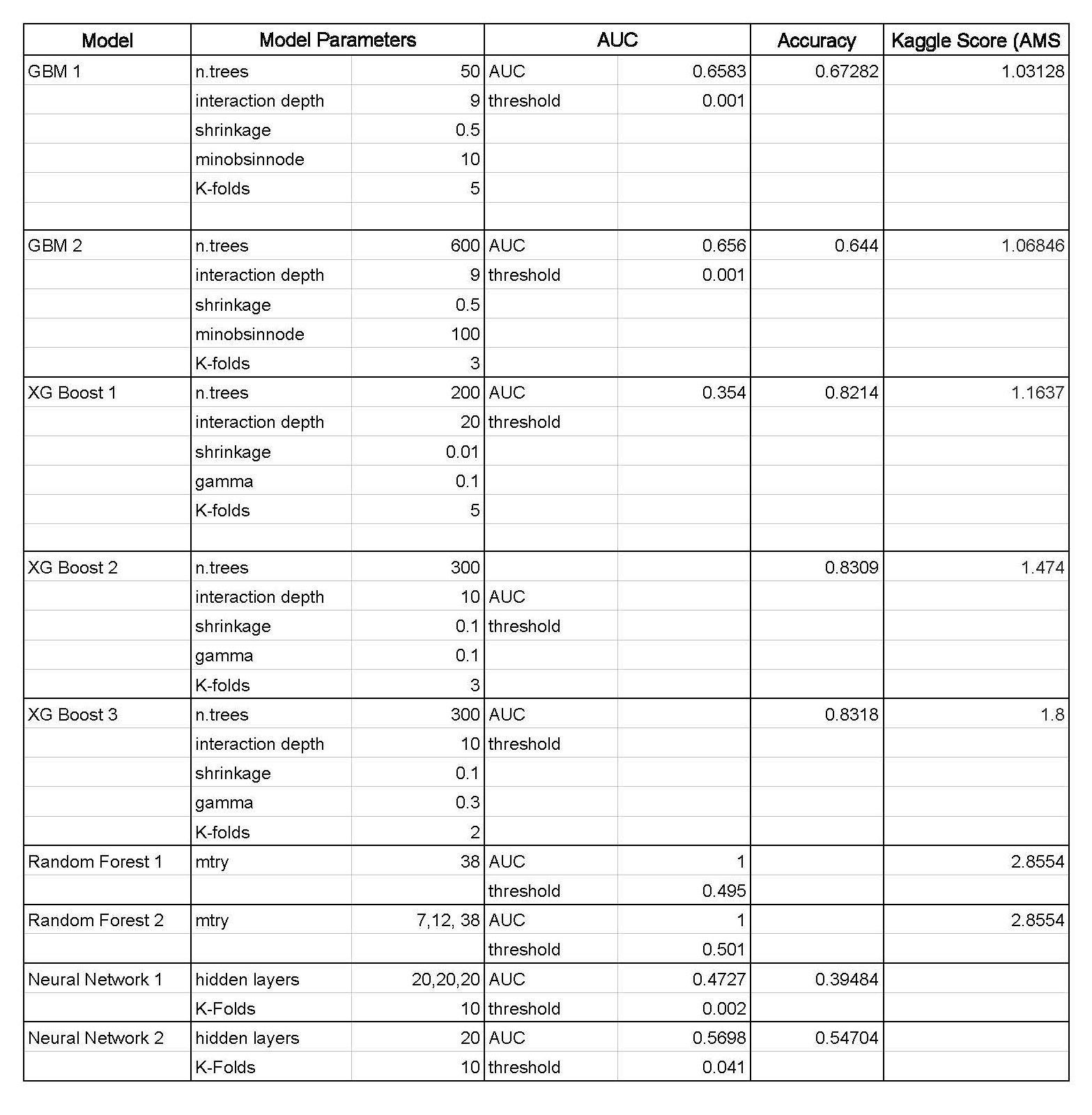
Model Comparison Sheet