
Introduction
House flipping, or buying a house and renovating it before selling it again, is a common technique used to turn up a profit in the real estate world. While renovation decisions are usually tailored to specific situations, our team found a way to inform these decisions intelligently, using machine learning models we trained on house selling data in Ames, Iowa.
In this collaborative project, our mission as the MASA team was firstly to train a machine learning model to be an optimal predictor for future house sale prices in Ames, Iowa. We then used our model to estimate the differences made by specific house features on sale prices, and in turn produced a practical guide for those looking to efficiently “flip” homes for a profit.
The Data
Kaggle provides a dataset with details about around 1500 homes sold in Ames, Iowa from 2006 to 2010. Each home in the dataset has 80+ features, such as lot area, amount of rooms, and kitchen quality. We explored, analyzed and carefully selected a subset of these features (along with engineering some of our own features) to simplify and sharpen the focuses of our subsequent models. We then used more formal techniques such as running a Lasso regression to further select our features, before feeding our finalized features into linear and tree-based models. Once we trained our most accurate model, we applied a Ridge regression in order to dissect each feature’s importance in an actual dollar amount, which serves as a practical, take-home guide for house flippers.
Exploratory Data Analysis (EDA)
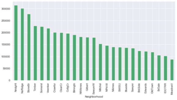
As we sought to hone in on the most interesting features in our dataset, we first noticed a positive skew in the sale price distribution of the overall data. To fix this, we took the natural log of the sale price; a more normal distribution resulted in this measure and was used as our new target variable in the subsequent models.
The rest of the 80+ variables were organized into 4 groups for ease of exploration.
An overview of the techniques we used for data analysis on these features groups is as follows:
- Dealt with missingness in features appropriately
- Visualized features and categories within categorical features with box plots, scatterplots, etc. to view their effects on sale prices; when uncertain about whether a feature made a difference in sale price, we performed ANOVA tests to test whether they made a significant difference. If they didn’t, we dropped these features or categories.
- Performed feature engineering where necessary
- Dummified categorical features in order to include them in linear models
Land and Exterior Features
House features relating to land include lot area, lot configuration (e.g. corner property), neighborhood, proximity to railroads, lot frontage, lot shape, alley presence, street type, land slope, and land contour. After analysis, we decided to impute values of 0 square feet where there were missing values for lot frontage. We got rid of the alley and street features since almost all homes had the same entry for them, and thus they wouldn't add differentiative power to our model. Land slope and land contour didn’t show enough of an impact on sale price, so we dropped them as well. The rest of the features were kept, with the anticipation that at least some would be impactful enough on sale price to end up in our final model.
As for house exterior features, we explored pool area, pool quality, porch area (broken into 5 types of porches: wood deck, open porch, enclosed porch, 3 season porch, screen porch), fence quality, and paved driveway material. Since only 8 homes in the data actually had pools, the pool quality column largely consisted of missing values, and so we dropped it. However, we kept the pool area feature since we figured the presence of a pool may still have a significant impact on a house’s value. Instead of retaining the square footage of these pools though, we converted the feature to a binary value: 0 for no pool, 1 for having a pool. The fence and paved driveway features were also reduced to binary, evaluating whether they are present at all or not.
House Structure & Utilities Features
The house structure features include Year Built, Year Remodeled, MSSubClass (type of property), MSZoning (zoning classification), Building Type, House Style, Overall Quality (of materials), Overall Condition (of the house), Roof Style (type of roof), Roof Material, Exterior 1st (covering on house), Exterior 2nd (covering on house), Masonry Veneer Type, Masonry Veneer Area, Exterior Quality (quality of the material), Exterior Condition (present condition of the material), and Foundation. Utilities features include Utilities (Type of utilities available), Heating (type of heating), Heating Quality, Central Air (central air conditioning), and Electrical System.
At first, we dealt with missing data points; there were 3 features with missing values Masonry Veneer Area (8), Masonry Veneer Type (8) and Electrical (1). After careful consideration, we assumed that the missing values resulted from human error. Electrical and Masonry Veneer Type were imputed with “NA”s and Masonry Veneer Area was imputed with 0s.
MSSubclass provides similar information to House Style and Building Type. Year Remodeled was assumed to have an effect on the overall quality of the house. Exterior 2nd and Exterior 1st were providing similar information as well. We decided to drop these features since they seem to add multicollinearity and don’t do well with predicting house prices accurately.
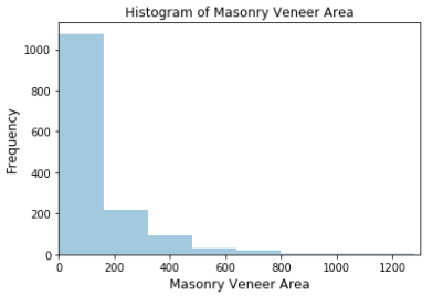
We created a histogram to view the distribution of the numerical feature Masonry Veneer Area (shown below), and evaluated its correlation coefficient with sale price (~ 0.43).
Since the distribution is skewed to the left and the area seems to be weakly correlated with price, we decided to drop this feature.
Again, for the categorical features in this subset of data, we created bar and box plots to view the distributions of categories within a feature and compared their means using ANOVA tests where a difference in means was doubtful. When no significant difference in sale price was found between categories, we engineered a feature that combines the categories. Electrical did not have any significant difference between its categories at all, so it was dropped. Central Air only had 2 categories and the categories were significantly different, so it was preserved without any feature engineering. Utilities had 99% of its data labeled as one category, so it was removed.
House Qualities & Garage Features
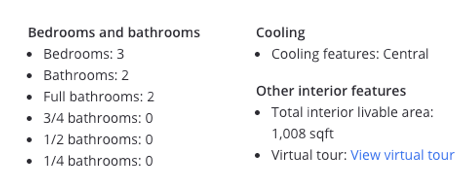
The variables in house qualities include first floor square feet, second floor square feet, above grade low quality square feet, above grade living square feet, full bathrooms, half bathrooms, basement full bathrooms, basement half bathrooms, bedrooms above grade, kitchens above grade, kitchen quality, total rooms above grade, functionality of the house, number of fireplaces, fireplace quality and fireplace year built. Since these qualities are mainly the fundamental descriptors of a house, we referred to Zillow.com to see how these characteristics are usually presented to users in order to retain information in our model that’s usually relevant to prospective home buyers. A current listing on Zillow of a house in Ames is shown below.
To correspond to this, we engineered the variables in our dataset as follows: livable square feet above grade, low quality square feet (mutually exclusive from livable square feet), total full bathrooms, total half bathrooms, total bedrooms, number of kitchens, kitchen quality, number of fireplaces, and functionality. The decisions on the functional categories were made by running a multiple linear regression on all of the house qualities variables and finding that fireplace quality only had about an $800 impact on price while kitchen quality’s impact was several thousands of dollars. Functionality was retained through domain inference that buyers would highly consider the current functionality of the house when making a valuation.
The variables describing garages in the dataset include type of garage (attached, detached, basement, built-in to house, more than one garage), year the garage was built, garage finish, garage condition, garage quality, garage area, and number of car bays. We split these variables into 3 different categories based on the information they contained:
- Quality of garage: garage finish, garage condition, garage quality, garage year built
- Type of garage: garage type
- Garage size: garage square feet, number of car bays
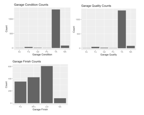
For garage quality, we retained garage finish, which describes the finish quality of the garage’s interior, and dropped all the other variables. We did this because garage finish had the greatest variance by far amongst the three variables, seen in the plots below. The year the garage was built was dropped because we inferred that buyers would put more weight on the year the actual house was built and only would only be concerned with the year the garage was built insofar as to discern the garage’s quality- information already contained in the garage finish variable.
The type of garage was retained as we hypothesized there would be a significant preference for attached garages.
Within the garage size category, square feet and car bay amount showed a very strong correlation coefficient of .9. We decided to drop garage square feet and retain the car bay amount as this seemed to offer an easier, more pragmatic model interpretation, while still retaining almost all the information given by garage square feet.
Basement and Miscellaneous Features
The basement categories in the dataset include the overall quality (how high the basement was in inches), the condition of the basement, the exposure (whether or not it was completely underground, or had access to natural sunlight), a few variables explaining whether or not the basement was finished, how much was left unfinished, the overall size of the basement in square footage, and whether or not the basement had a bathroom. For the most part, the variables explaining the basement finish were very highly correlated with each other, and after exploring the variables further, we found through ANOVA testing that only the first variable, which told us whether the basement was finished or not, mattered. We kept quality, condition, and exposure after similar analysis, and the overall square footage of the basement seemed to correlate with sale price as well. The amount of bathrooms didn’t have an effect on the overall sale price, but the presence of a bathroom did. This, we decided, had more to do with the presence of a bathroom in the house itself, rather than the basement specifically. We also wanted to explain our findings in a way similar to a Zillow listing, where all the bathrooms were listed as a grand total, not specific to location. So we added the basement bathrooms to the total bathrooms, and dropped those two columns.
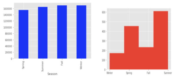
There were a few miscellaneous categories to look at as well. Miscellaneous features and their values were present as variables, but were only present in 4% of the houses - less than 60 in our dataset of 1460. Furthermore, most of the houses with extra features had sheds, and the remaining categories had very few entries in our dataset (tennis courts, a second garage, etc.) Since that variable was so sparse, and the values would have likely been reflected in the overall value of the house, we dropped both columns. Sale condition and sale type were interesting, in that the way the house was sold did affect the sale price. Buying from a foreclosure, or from a low interest contract, for example was correlated with a lower sale price. We thought this information would be useful to buyers looking to get a big house for cheaper, even though the data was sparse, so we left those columns in. Finally, the time series data available didn’t affect house prices much at all, to our surprise. We saw no large changes in price from 2006 - 2010, even though the housing crisis occurred right in the middle of this range. We saw that as a testament to the stability of the housing market in Ames. And while we expected seasonality, the housing prices were relatively stable across months as well. We did note the overall count of houses was very different across the spring and summer months, relative to the fall and winter months. We kept month as a variable so that our clients would hopefully be able to use this information to flip houses during the busier months, where their houses would be more likely to sell due to the higher demand.
Feature Selection with Lasso Regression
Once our initial round of EDA was complete, we ran a lasso regression with our compiled features in order to further narrow down and modify the features that would make it to our final model. We used the lasso method since it would reduce the beta values of features with little to no importance (impact on sale price) to 0, thus eliminating them. In order to find the optimal lambda value, we performed a randomized grid search which yielded a result of 4.4e-5 with an R^2 of .87934. The high R^2 validated the use of this model to further cut and modify features. It should also be noted that all ordinal and categorical variables were dummified as to not imply ratio distances between values (average to good could be a greater or smaller distance than good to excellent).
We converted our beta values into marginal percent impact on the log sale of price and modified our features in the following ways:
- Continuous variables with betas of 0 were cut completely
- Continuous variables with betas under 2 with low possible values were cut (such as extra rooms which had a beta value of .88 and a max of 7 and a mean of 3).
- Categorical variables where each value was under 2% were cut completely
- Categorical variables where some but not all categories were under 2% were converted to less specific groups- for instance, some variables’ only significant values were “excellent” in which case the values were changed to “excellent” and “other”.
The complete results of the lasso can be found in the linked Github; we have included a preview below to depict the above processes:
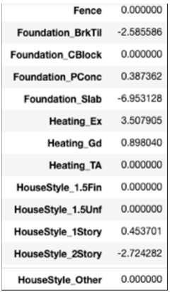
For the above variables, the categorical variable fence was cut out completely. The foundation variable was changed to Foundation_BrkTill, Foundation_Slab and other, heating was changed to Heating_Ex or other and HouseStyle was changed to HouseStyle_2Story or other. We implemented these changes to produce a finalized dataframe for our predictive model.
Tree-Based Machine Learning Models
After feature reduction, we ran 2 tree-based models on our data to predict sale prices: random forest and gradient boosting. Grid search was performed with 5-fold cross validation to optimize the hyperparameters in both models. For random forest, the number of leaves, minimum sample to split, max depth of tree and number of trees were optimized. Maximum depth, maximum features, minimum impurity decrease, minimum sample split and number of estimators were optimized for the gradient boosting model, with 5-fold cross validation and a learning rate of 0.01, subsample of 0.7 and scoring criteria as r-squared. The optimized parameters were used to train the model. Our gradient boosting model (R2 = 0.96, RSME = 0.13) performed slightly better than our random forest model (R2 = 0.94, RSME = 0.15) model, presumably due to the linearity of the data, which works well with gradient boosting.
Feature Importances
After we ran our Gradient Boosting model with our optimized parameters that we gained through our Grid Search, we were able to get a list of the top 11 most important features in determining house price, which are as follows:
- Ground Floor Living Area
- Overall Quality (of the materials used in the house)
- Garage Cars (how many cars the garage can fit)
- Total Basement Square Footage
- Kitchen Quality
- Number of Full Bathrooms
- Year Built
- Fireplaces
- Exterior Quality
- Lot area (size of the overall property, yard included)
- Basement Quality (height)
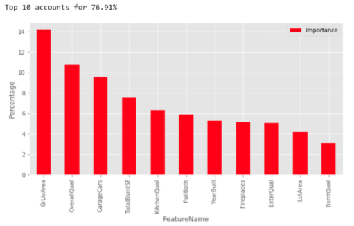
Together, this information accounted for 77% of the total decisions our model made about housing prices. We knew it was important to communicate these features to our target audience, and we wanted to do so in a way where they could see the dollar value of making certain improvements in a home, or buying a home of a certain type. To do this, we first used our Gradient Boosting model to predict the housing prices on our test data set. From this, we ran a ridge regression model on our features verses these test prices, with the intention of being able to assign dollar figures to different improvements based on the beta coefficients we received from the model.
Conclusions
From this, we accomplished our goal, and could draw some very interesting conclusions about what a house flipper would have to do in order to get the most value out of the house they are flipping. To start, there were certain features that couldn’t be altered easily, so we advised our clients to buy houses that already had great values for the features. These were the year built (newer houses sell for more), the basement size and height (since a large underground renovation would likely cost more than it was worth), and the lot area (since the houses were likely sold on a specific lot). That left a lot of variables for our house flippers to play with, fortunately, and we could advise them on the improvements they could make that would net them the most profit. Extending the garage, for example, would add $10,000 for every additional car that the renovated garage could fit. Adding another full bathroom anywhere in the house also correlated with a $10,000 increase in sales price. Improving the kitchen to that of an excellent quality, rather than just a good or a typical quality, would improve the sale price of the house by $20,000. The overall quality of the house, however, had to be approached with caution. On a one to ten scale, improving the overall quality of the house to anything at a level six or lower would not cause improvements in the overall sale price. Once you reached level seven and above, however, house prices increased dramatically, even reaching levels above those of the kitchen improvements. So our greatest recommendation was to invest in high quality materials to put in the house, so that house flippers would see the greatest return on investment.
Topics from this blog: Machine Learning python machine learning Student Works