Caterpillar Tube Assembly Pricing

Contributed by by Adam Cone and Ismael Cruz. They are currently in the NYC Data Science Academy 12 week full time Data Science Bootcamp program taking place between April  to April 1st, 2016. This post is based on their Capstone Project due in the final week of the program).

Introduction

Our challenge came from a Caterpillar-sponsored Kaggle competition that closed in August, 2015. 1,323 teams competed.

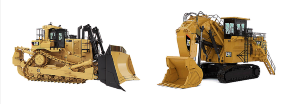
Caterpillar Inc., is an American corporation which designs, manufactures, markets and sells machinery, and engines. Caterpillar is the world's leading manufacturer of construction and mining equipment, diesel and natural gas engines, industrial gas turbines and diesel-electric locomotives. Caterpillar's line of machines range from tracked tractors to hydraulic excavators, backhoe loaders, motor graders, off-highway trucks, wheel loaders, agricultural tractors and locomotives. Caterpillar machinery is used in the construction, road-building, mining, forestry, energy, transportation and material-handling industries. (from Wikipedia)

Caterpillar relies on a variety of suppliers to manufacture tube assemblies for their heavy equipment. Our task was to predict the price a supplier will quote for a given tube assembly.

Objective: predict the quote price of a tube assembly, given past tube assembly price quotes

We programmed in Python using Jupyter Notebook. All our code is available on github here.

Data

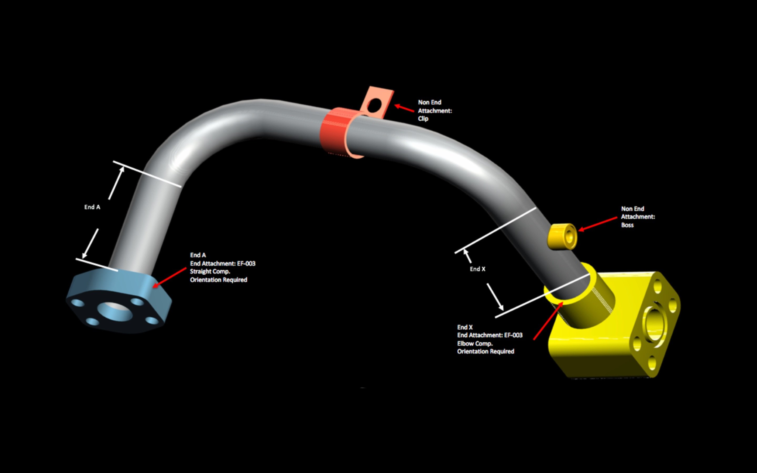
A tube assembly consists of a tube and components. There are 11 types of components and a tube assembly can have any of these types in various quantities, or no components at all. In addition, the tube can be bent multiple times with a variable bend radius, and the tube ends can be prepared in various ways.

Our original data consisted of 21 different csv files. Each file contained information about different aspects of the tube assemblies. For example, tube.csv consisted of tube-specific information, such as the tube length, how many bends the tube had, the tube diameter, etc. We imported each of the csv files into our notebook as independent pandas data frames.

Our first thought was to simply join the different data frames into a single data frame for all analysis. However, this would have resulted in a data frame with many missing values, since most tube assemblies lacked most components. For example, tube assembly TA-00001 had 4 components: 2 nuts and 2 sleeves. TA-00001 had no adaptor. The adaptor data frame had 20  adaptor-specific variables (columns), for example adaptor_angle. A left join of our tube data frame to our adaptor data frame would mean that TA-00001 would have a column for adaptor angle, even though TA-00001 has no adaptor component. This would result in a missing value in this column. Furthermore, similar missing values, would be problematic to impute, since their origin is structural and not random. Therefore, instead of joining all the data frames, we engineered new features to add as much information from the components data frames, while introducing no missing values in the train and test data frames.

Although we couldn't join most of the 21 csv files, we did join the tube data frame to the training set data frame without introducing new missing values. To get information from the remaining csv files, we engineered 3 new features that summarized data about the components. For example, with one new engineered feature, we saw that TA-00001 has two types of components, although we wouldn't see what these components are, let alone details of the components available in the related csv files. Later, we added 11 additional features: each a count a particular component type of each tube assembly. For example, with the 11 new engineered features, we see that TA-00001 has 2 nuts and 2 sleeves. Because we weren't sure whether these additional 11 columns would be useful in predicting tube assembling prices, we built two data frames for model fitting: basic data frame (did not include 11 new feature engineered columns) and components data frame (includes 11 new feature engineered columns).

For missing values in our categorical data (e.g. tube specifications), we added a new NaN level, obviating the need to impute or throw away observations. The only numerical missing values were in bend_radius: 30 total in all 60,448 test and training observations (~0.05%). We imputed these bend_radius values with the mean bend_radius, since we found no pattern to the missingness and there were relatively few missing values. Next, we converted our categorical variables to dummy variables, where each factor level became a column with values of either 0 or 1. Lastly, we converted the quote dates into days after the earliest date.

After the above changes, we had two complete (i.e. no-missingness), entirely numerical data frames to use for model fitting and prediction: basic (158 columns) and components (169 columns).

Modeling

We used three tree-based models:

1. decision trees,
2. random forests, and
3. gradient boosting.

We fit each model to each of the two training sets (basic and components). We compared each model's performance on the basic and components data frames, and against the other two tree-based models. We expected better predictions from the models fitted to the components data frame than models fitted to the basic data frame. In addition, we expected gradient boosting to outperform random forests, and that both would outperform decision trees.

For our decision trees, we made four attempts, each time changing the tuning parameter grid. These were labeled as A1, A2, A3, and A4 on the x-axis of the graph below. The performance of each decision tree was measured using the percentage of Kaggle teams outperformed. In the figure below, we see that from A1 to A3, the models fitted with the components data frame outperformed those fitted with the basic data frame. The tuning parameters for A1-A3 were min_samples_leaf (the minimum number of observations in a node) and min_samples_split (the minimum number of observations necessary to split a node).

For A4, we increased the computation time, but changed the tuning parameter to max_leaf_nodes (the maximum number of nodes in the final tree), and left min_samples_split and min_samples_leaf as defaults. Despite the increased computation time, A4 performed worse than any of the previous attempts. Furthermore, the performance of the model fitted to the components data frame dropped in comparison to the performance of the model fitted to basic frame.

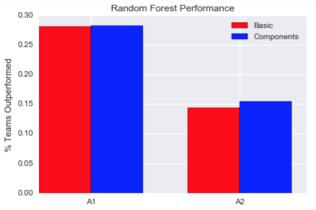
For our random forests, we made two attempts, each time changing the tuning parameter grid. These were labeled as A1 and A2 on the x-axis of the graph below. In the figure below, we see that for A1, the model fitted with the components data frame outperformed that fitted with the basic data frame. The tuning parameters for A1 were min_samples_leaf and min_samples_split, and we fixed the n_estimators (the number of trees) at 100.

For A2, we increased the computation time, increased n_estimators to 1,000, changed the tuning parameter to max_leaf_nodes, and left min_samples_split and min_samples_leaf as defaults. Despite the increased computation time, A2 performed worse than A1.

For our gradient boosting, we made two attempts, each time with a different tuning parameter grid. These were labeled as A1 and A2 on the x-axis of the graph below. In the figure below, we see that for A1, the model fitted with the components data frame performed identically to that fitted with the basic data frame. The only tuning parameter for A1 was learning_rate: n_estimators was fixed at 100 and max_leaf_nodes was fixed at 2 (other parameters were defaults). max_leaf_nodes fixed at two corresponds to 'stumps': trees with exactly one split.

For A2, we increased the computation time, increased n_estimators to 1,000, changed the tuning parameter grid to three values of learning-rate between 0.001 and 0.01, set max_leaf_nodes to 2, and left other parameters as defaults. Despite the increased computation time, A2 generated nonsensical results. Specifically, A2 on both basic and components data frames predicted multiple negative costs for tube assembly quotes.

Finally, the highest-performing models for each tree-based method (all fitted to the component data frame) are compared in the bar plot below. The random forest and the decision tree performed similarly, and both outperformed gradient boosting.

Lessons

We anticipated that the models fitted to the component data frame would outperform the models fitted to the basic data frame. We did not consistently observe this. For the decision tree, A4 showed better results for the basic data frame than for the component data frame. For gradient boosting, A1 showed identical performance for models fit on the data frames. Neither of the A2 gradient boosting models had intelligible results at all. Therefore, we conclude that our additional feature engineering did not consistently improve prediction accuracy. Although in 5 of our 8 documented modeling attempts, models fit to the components data frame performed better, this improved performance seemed to also depend on the type of model used and the tuning parameters chosen.

Furthermore, we anticipated that gradient boosting would outperform random forests and decision trees. We did not observe this. In fact, our best gradient boosting model outperformed ~8% of teams, whereas our worst decision tree outperformed ~12% and our worst random forest outperformed ~14%. Again, our gradient boosting model even generated nonsensical results: decision trees and random forests never did. The A2 gradient boosting method predicted nonsensical results in the form of negative numbers for both data frames. The interpretation of these results is that the supplier would pay Caterpillar for each tube assembly ordered.

In our final decision tree and random forest attempts, performance decreased sharply when we chose a different tuning parameter, despite investing more computation time in searching the parameter grid. This suggests that choice of tuning parameter can be more important for decision trees than  raw computational power in the tuning process.

Similarly, the performance for A1 gradient boosting was identical for both the basic and components data frames. We suspect that by choosing 100 'stumps' (trees with exactly one split), we were able to access at most only 100 features in our feature space (158 for basic; 169 for components). So, it's possible that the additional 11 features in the components data frame were not used at all in the gradient boosting algorithm, so the decision trees, and therefore predictions, were identical in both cases. In this case, by using fewer stumps than features in our feature space, we limit the algorithm's use of the data.

Finally, we logged several of our parameter tuning runs. For example, our log for the decision tree model using the components data frame is illustrated in the table below. We found this logging process helpful in diagnosing the changes in performance of each of the models.

Improvements

With more time to work on this project, we would be even more diligent and detailed in our logging of parameter tuning attempts. Specifically, we would also log the date, time of day, computation duration, R^2 of test and train, and parameter grid ranges for each parameter.

Also, we would like to tune our parameters based on the Kaggle metric: the Root Mean Squared Logarithmic Error (RMSLE):

not on the coefficient of determination, which is the default tuning metric in the Python scikit-learn library. We hope that by using the RMSLE, we would achieve better results by creating each split in each tree with specific sensitivity to the Kaggle competition.

Finally, we would like to try to use Spark to parallel process and improve our computation time.